Optimization for Machine Learning: Lasso Algorithm and Related Problems

Optimization for Machine Learning

INSIGHTS
$
SQL
€
?
Optimization for Machine Learning
Y
CLOUD
SECURITY
BIG DATA
PATTERNS
Prof. Giuseppe Calafiore
f
Dept. Electronics and Telecommunications
Politecnico di Torino
SOCIAL
APPS
PLATFORM
-
1
1
MEMORY
PEOPLE
PEOPLE
CARE
INTERNET OF THINGS
G.C. Calafiore (Politecnico di Torino)
4
SPEED
STORAGE!
AZURE
300
000
BYOD?
600
DEVELOPERS
WEB
- MAGIC
DEVICES

Algorithms for the Lasso and Related Problems

1 / 16LECTURE 6
Algorithms for the Lasso and related problems
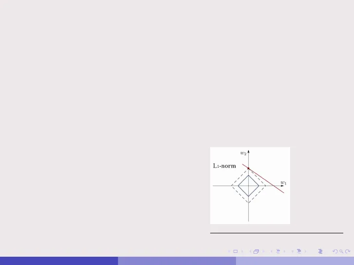
W21
L1-norm
-
-
-
-
>
/
1
-
G.C. Calafiore (Politecnico di Torino)
5

Outline of Lasso Algorithms

2 / 16Outline
1
Algorithms for the Lasso
2
Coordinate descent for the Lasso
G.C. Calafiore (Politecnico di Torino)
=
3 / 16Algorithms for the Lasso
G.C. Calafiore (Politecnico di Torino)
=
4 / 16Algorithms for the Lasso
. We recall that the Lasso can be encountered in two equivalent forms.
. The Lagrangian, or penalty, form:
min y - 0 w|2 + \| w |1
w
. The constrained form:
min
w
lly - Tw |2
s.t .:
w|1 St.
. Both forms can be expressed as convex QPs (quadratic programming).
. For example, the penalty form is expressed equivalently as
min
W, S
y - Qw|2 + 2=1 Si
s.t .:
-Si ≤ wi ≤ Si,
i=1, ... ,d.
G.C. Calafiore (Politecnico di Torino)
5 / 16Algorithms for the Lasso
. A classical algorithm fo solving the Lasso is the so-called Least Angle
Regression (LAR) algorithm:
B. Efron, T. Hastie, I. Johnstone, and Robert Tibshirani, "Least angle
regression," Annals of Statistics, Vol. 32, No. 2, pp. 407-499, 2004.
. LAR computes entire path of solutions, i.e., solutions for all ).
State-of-the-Art until 2008.
. Later, Coordinate Descent (CD) methods emerged as an efficient alternative:
T.T. Wu and K. Lange, "Coordinate descent algorithms for Lasso
penalized regression," The Annals of Applied Statistics, Vol. 2, No. 1, pp.
224-244, 2008.
. CD methods coded into some widely used packages, such as the R package
glmnet.
. The ADMM is yet another approach to Lasso solution.
. Many other approaches, e.g., FISTA (Beck and Teboulle, 2009).
G.C. Calafiore (Politecnico di Torino)

Coordinate Descent for Lasso

6 / 16Coordinate descent for the Lasso
. We next consider the Lasso in the penalty form
min f (w) =
WERd
2
1
-y - 0 w|2 + w|1
and discuss a coordinate minimization method for its solution.
. We observe that the Lasso objective is convex but nondifferentiable.
. However, it possesses the convex and "differentiable plus separable"
structure
f(w) = fo(w) +>>
d
i=1
vi(wi),
where fo(w) = Ally - Tw|} and vi(wi) = |wil.
. Therefore, a simple sequential CD method is guaranteed to converge to the
global optimum for the Lasso!
G.C. Calafiore (Politecnico di Torino)
=
7 / 16Coordinate descent for the Lasso
. If w is the current point, then the i-th coordinate minimization problem
takes the form (all but the i-variable are fixed to the values in w, and we
minimize with respect to w;)
min
w; ER
1
2
|4;w; - y( 1) |2 + \wil + x|w( -; ) |1,
where pi is the i-th column of $ , W(-i) is a vector obtained from w by
fixing the i-th entry to zero, and y() = y - ¢ w(-i).
. Since | W(-i) |1 does not depend on the w; variable, we see that the
coordinate-wise optimization problem can be rewritten equivalently as
min fi(x) =
x
1
2
Ilxix - y (1)|2 + x|x|,
(1)
where x E IR is the variable.
. We next show how to compute in closed form the optimal solution of (1).
G.C. Calafiore (Politecnico di Torino)
8 / 16Coordinate descent for the Lasso
min fi(x) =
x
1
2
alloix - y (1)|12 + x|x|,
. Use the following "trick": |x|= maxse[-1,1] sx and rewrite the problem as
minx }(pix -y(i)(xix - y(1) + \ maxse[-1,1] SX =
2(xix - y(1) (xix - y(1) + \sx =
minx maxse[-1,1]
maxse[-1,1] minx
1
2
(pix-y(1)(pix-y(1) + \sx,
where the last passage (swap of min and max) is justified by the fact that
the function is convex-concave in x and s, respectively.
. We can now solve the inner minimization analytically, by observing that
min
x
1
2
(xix - y(i) (xix - y(i) + \sx
is achieved when the gradient (derivative) w.r.t. x is zero, i.e.
X
1
2
(x2114;112-2×4; y(1) + |y(1)}) + \sx
= x|pill2-4; y(1) + s = 0.
G.C. Calafiore (Politecnico di Torino)
=
9 / 16Coordinate descent for the Lasso
. We thus obtain that the minimum w.r.t. x is achieved at
x*(s) =
1
112
(6; y(1) - \s),
Ilpill2
whence, substituting the optimal value for x, we obtain (after some
manipulation):
min
x
1
2
-(xix - y(1) (xix - y(1) + \sx
= g(s) = -
1
2 |4: 13
12
s-
2
+
16; y(1)
114:112
112
S +
1
2
(1)(1)13
(i)
(6; y (1)2).
114:112
. The above function in s is a parabola with vertex in v = 0; y(1)/A. Since we
need to maximize g(s) over the interval [-1, 1] we have that the vertex is
the optimum point if |v| < 1, that is s* = 0; y(1)/> if |4; y (i) <1.
Otherwise, the optimum is achieved at one of the extremes of the interval,
in particular in s* = sgn(p, y(i)).
G.C. Calafiore (Politecnico di Torino)
10 / 16Coordinate descent for the Lasso
· Summarizing, we have
S
*
=
6 ; y (1)/ >
T
sgn(pi y(i))
if | 4 ; y (1 ) | < >
if | 6 y ( 1) > >
and, consequently
∗
x
=
ϕi
2
2
=
0
4; y (i)
−
114; 112
12
λ
Il 4:112
if | 4; y (1 ) < 1
if | 4 ; y ( 1) | > >,
where §i = sgn(4; y (i).
.
Observe that
T
Zi =
4;y (1)
2
corresponds to the solution of the problem for > = 0 (i.e., the LS solution).
=
G.C. Calafiore (Politecnico di Torino)
11 / 16
1
(6; y (1) -15*)Coordinate descent for the Lasso
. Observe that if
|0y |00 ≤ 1
then x = 0 is an optimal solution for the Lasso.
. The proof of this fact arises from the consideration that if we start from
x = 0 and apply a coordinate descent method, then the variable updates will
all remain zero, since y() = y - ¢ "w( -; ) = y for all i (due to the fact that
W(-i) = 0), and hence
10; y(1) =|4; y| < >, i = 1, . , d.
G.C. Calafiore (Politecnico di Torino)
=
12 / 16Coordinate descent for the Lasso
. The univariate Lasso solution can be expressed in terms of the so-called
soft-thresholding function:
w= = sthr/|4;|13(zi),
where zi =
6; y (1)
16:12, and sthr is the soft threshold function:
sthr.(z)=sgn(z)(|z|-ơ)+
strhg(z)1
/
/
-0
0
6
2
/
=
G.C. Calafiore (Politecnico di Torino)
13 / 16Coordinate descent for the Lasso
. CD methods for the Lasso come in various flavors, see, e.g.,
T.T. Wu and K. Lange, "Coordinate descent algorithms for Lasso
penalized regression." The Annals of Applied Statistics, vol. 2, n. 1,
pp. 224-244, 2008.
J. Friedman, T. Hastie and R. Tibshirani, "Regularization Paths for
Generalized Linear Models via Coordinate Descent." J. of Statistical
Software, vol. 33, n. 1, 2010.
G.C. Calafiore (Politecnico di Torino)

Summary of Coordinate Descent for Lasso

14 / 16Coordinate descent for the Lasso
Summary
. Solve the Lasso problem by (cyclic) coordinate descent: optimize each
variable separately, holding all the others fixed. Updates are trivial. Cycle
around till coefficients stabilize.
. Do this on a grid of ) values, from Amax down to Amin (uniform on log
scale), using warms starts.
. Can do this with a variety of loss functions and additive penalties.
· Coordinate descent achieves dramatic speedups over all competitors, by
factors of 10, 100 and more.
G.C. Calafiore (Politecnico di Torino)
=
15 / 16Coordinate descent for the Lasso
Tricks
. Active Set Convergence: after a full cycle through the d variables, we can
restrict further iterations to the active set (i.e., the set of nonzero variables)
till convergence, plus one more cycle through all d to check if active set has
changed: if it changed, we continue the iterations on the new active set, and
so on; otherwise we finished.
Helps when d >> N.
. Warm Starts: we fit a sequence of models from Amax down to Amin.
Xmax is the smallest value of \ for which all coefficients are zero. Solutions
don't change much from one X to the next. Convergence is often faster for
entire sequence than for single solution at small value of ).
G.C. Calafiore (Politecnico di Torino)
=
16 / 16