Fundamentals of Automatic Control: Motivations, Concepts, and Examples

UNIVERSITÀ DEGLI STUDI DI TRIESTE

Fundamentals of Automatic Control: Module Content

UNIVERSITÀ DEGLI STUDI
DI TRIESTE
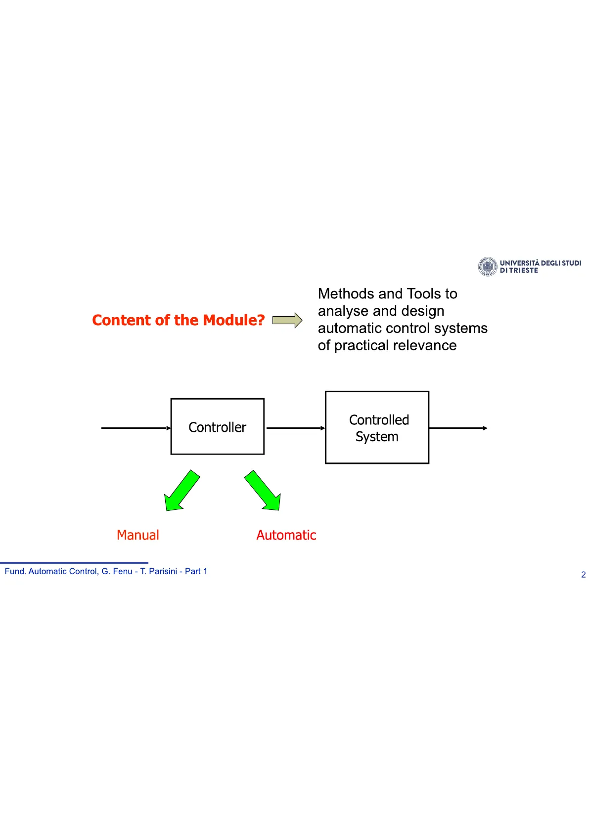
Content of the Module?
Methods and Tools to
analyse and design
automatic control systems
of practical relevance

Controller
Controlled
System
Manual
Automatic
Fund. Automatic Control, G. Fenu - T. Parisini - Part 1
2

The Control Problem

UNIVERSITÀ DEGLI STUDI
DI TRIESTE
To impose a given time-trajectory to one or more specific variables of an
engineering system by acting on other variables that influence the
behaviour of the system itself

Controller
Controlled
System
Manual
Automatic
Fund. Automatic Control, G. Fenu - T. Parisini - Part 1
3

Example: Speed Control

UNIVERSITÀ DEGLI STUDI
DI TRIESTE

Wind
Road slope
Desired
speed
Accel.
Actual speed
Driver
Car (load)
Brake
Speed Meas.
"closed-loop" strategy
Effective in the
presence of
uncertainty
Fund. Automatic Control, G. Fenu - T. Parisini - Part 1
4

Control Theory Brief Tour (Youtube)

UNIVERSITÀ DEGLI STUDI
DI TRIESTE
https://www.youtube.com/watch?v=IBC1nEg0 nk
GB
YouTube
Search
Q
How do you get a system to do what you want?
Distillation Column
Autonomous Driving
Temperature Control
Condenser
FOR
Reboiler
Bettom letes
0
Control
Theory
Fund. Automatic Control, G. Fenu - T. Parisini - Part 1
5

Closed-Loop Control Strategies

UNIVERSITÀ DEGLI STUDI
DI TRIESTE

w +
e
u
y
C
Se
ym
M
· Se : system to be controlled
· C : controller
· 0 : system's parameters
· y : controlled variable (output)
· u : control variable (accessible to the controller)
· d : disturbance
· w : reference variable (set-point)
· e : error
· ym : measured output
Fund. Automatic Control, G. Fenu - T. Parisini - Part 1
6

Requirements for an Analog Continuous-Time Control System

UNIVERSITÀ DEGLI STUDI
DI TRIESTE
The basic requirement is:
y(t) ~ w(t)
Introducing the error variable e(t) = w(t) - y(t) , the above requirement
becomes:
e(t) ~ 0 in all situations "of interest"
Without loss of generality, we focus on the continuous-time case. The
discrete-time case is perfectly analogous
Fund. Automatic Control, G. Fenu - T. Parisini - Part 1
7

General Requirements of Control Systems

UNIVERSITÀ DEGLI STUDI
DI TRIESTE

• (A) Static precision
  + In equilibrium conditions
• (B) Dynamic precision
  + Speed of response
  + Damping of possible oscillations
  + Capability of tracking fast-varying
  reference variables w(t)
• (C) Insensitivity to disturbances
  + Capability of rejecting a
  disturbance d(t)
• (D) Robustness
  + (A), (B), (C) in the presence of
  uncertain system's parameters e

y(t)
w(t)
y'(t)
y""(t)
t
y(t)
w(t)
y'(t)
d(t)
Fund. Automatic Control, G. Fenu - T. Parisini - Part 1
t
8

Example 2: Position Control

UNIVERSITÀ DEGLI STUDI
DI TRIESTE

Mechanical
system
2.0
Fa
M
E
F
Fe
· Control input: external force F
· Controlled output: position of the cart x
· Reference output: desired position w = xº
· Elastic spring force: Fe = kx
· Damper viscous friction force: Fa = hx
Fund. Automatic Control, G. Fenu - T. Parisini - Part 1
9

Static Modelling

UNIVERSITÀ DEGLI STUDI
DI TRIESTE

F = kx
8
F
Fa
x
F
F
Fe
1
8
F
k
output
input
Equilibrium of the forces
in static conditions
Fund. Automatic Control, G. Fenu - T. Parisini - Part 1
10

Open-Loop Control Strategy

UNIVERSITÀ DEGLI STUDI
DI TRIESTE

0
F
Controller
k nominal value of the
spring constant
Controlled System
Controller
0
F
8
x
1
k
x =
一 九 一 た
e = x - x = x 1
k
W )
Fund. Automatic Control, G. Fenu - T. Parisini - Part 1
11
F = kxº

Open-Loop Control Strategy (contd.)

UNIVERSITÀ DEGLI STUDI
DI TRIESTE
- In nominal conditions k = k
e=0
- In uncertain conditions k + k
e=1º #0
Ak
△k)=k-k =0
uncertainty
There is no way to compensate for the uncertainty by an
open-loop control strategy
Fund. Automatic Control, G. Fenu - T. Parisini - Part 1
12

Closed-Loop Control Strategy

UNIVERSITÀ DEGLI STUDI
DI TRIESTE

Controller
?
F
1
8
k
Let us opt for a proportional control strategy:
F= a (xº-x), a>0
e
Fund. Automatic Control, G. Fenu - T. Parisini - Part 1
13

Closed-Loop Control Strategy (contd.)

UNIVERSITÀ DEGLI STUDI
DI TRIESTE
Suppose xº # 0 :
x = F = +a (xº - x) )
1
k
1
L
a/k
1+a/k
a (1+2) = 7º
e = xº - x =
1
1 +a/k
200
- In nominal conditions k = k
e=0
- In uncertain conditions k + k
e~0 if a >> kmax
Fund. Automatic Control, G. Fenu - T. Parisini - Part 1
14

Dynamic Modelling

x
F.
E
F
Fe
F'
a
F!
UNIVERSITÀ DEGLI STUDI
DI TRIESTE
F = a (xº - x) , a>0
e
The effects of mass, spring, and
damper are not negligible, and
dynamic behaviours such as
oscillations may occur
L
Models capturing the
dynamic modes of
behaviour are clearly
necessary
Fund. Automatic Control, G. Fenu - T. Parisini - Part 1
15

Dynamic Modelling (contd.)

UNIVERSITÀ DEGLI STUDI
DI TRIESTE
sum of all external forces = Mx
F - kx - hx = Mx
L
Mx + hx + kx = F
F
8
Fund. Automatic Control, G. Fenu - T. Parisini - Part 1
16

Open-Loop Control Strategy

UNIVERSITÀ DEGLI STUDI
DI TRIESTE

0
F
x
Mx + h& + kx = kxº
x(0)
*(0)
dynamic
terms
constant
initial
conditions
condition for
static equilibrium
Fund. Automatic Control, G. Fenu - T. Parisini - Part 1
17

Open-Loop Control Strategy (contd.)

UNIVERSITÀ DEGLI STUDI
DITRIESTE
Livescripts in MS Teams: see Part 1:
CART_OPENLOOP_CONTROL
From differential equations theory:
Mx + hx + kx - kxº
constant term due to open-loop control
MX2+hX+k=0
X1,12
polynomial algebraic equation
roots
- If X1, 12 are real
x(t) = c1e11t + C2e12+ + C3
- If X1, 12 are complex conjugate, that is >1=o +jw, 12= 0 - jw
L
x(t) = c4etcos(wt +c5) +c6
Fund. Automatic Control, G. Fenu - T. Parisini - Part 1
18

Open-Loop Control Strategy (contd.)

UNIVERSITÀ DEGLI STUDI
DI TRIESTE

x0 (1 - Ak
k
x(t)
static precision
X1, 12 complex conjugate
X1, 12 real
t
L
By the open-loop control strategy the dynamic behaviour
cannot be modified since it only depends on the system's
parameters M, k, h and not on the controller. Hence
dynamic precision cannot be modified by the controller
Fund. Automatic Control, G. Fenu - T. Parisini - Part 1
19

Closed-Loop Control Strategy

UNIVERSITÀ DEGLI STUDI
DI TRIESTE
Let us use again a proportional closed-loop control strategy:
F=a (xº-x), a>0
e
Mx + hx + kx = F
e
F
8
a
+
Fund. Automatic Control, G. Fenu - T. Parisini - Part 1
20

Closed-Loop Control Strategy (contd.)

UNIVERSITÀ DEGLI STUDI
DI TRIESTE
Plugging in the proportional control scheme we get:
Livescripts in MS Teams: see Part 1:
CART_CLOSEDLOOP_P_CONTROLLER
Mx + hi + kx = a(xº -x)
L
Mä + h& + (k+a)x=axº
the constant term of the algebraic
equation is influenced by the controller
gain &
4
MX2 + hX +(k+a)
= 0
11, 12
polynomial algebraic equation
roots
The roots A1, A2 can be modified by choosing & !!
Fund. Automatic Control, G. Fenu - T. Parisini - Part 1
21

Closed-Loop Control Strategy (contd.)

UNIVERSITÀ DEGLI STUDI
DI TRIESTE

x(t)
static precision
0.1
a
02
k +a
a
t
L
. The dynamic precision also depends on the choice of the
control gain
Static and dynamic requirements are in contrast with each
other: better static precision implies worse dynamic precision
Fund. Automatic Control, G. Fenu - T. Parisini - Part 1
22

A Different Closed-Loop Control Strategy

UNIVERSITÀ DEGLI STUDI
DI TRIESTE
Let us now opt for a proportional/derivative control scheme:
F = a (xº - x) + 3= (xº - x) , a, B > 0
Mä + hx + kx = a(xº -x) - Bx
Mä+(h+B)+(k+a)x=axº
Livescripts in MS Teams: see Part 1:
CART_CLOSEDLOOP_PD_CONTROLLER
the first-order term of the algebraic
equation is influenced by the derivative
controller gain 3
4
MX2+((h+B)\+(k+a)=0
X1,12
polynomial algebraic equation
roots
The roots X1, 12 can be modified
by choosing a, B !!
the constant term of the algebraic
equation is influenced by the
proportional controller gain &
Fund. Automatic Control, G. Fenu - T. Parisini - Part 1
23

Example 3: Tank Level Closed-Loop Control

UNIVERSITÀ DEGLI STUDI
DI TRIESTE

Hydraulic
system
qe
level sensor is needed
to close the control loop
h
qu
d
A
· Control input: input flow-rate qe
· Controlled output: level of liquid in the tank h
· Reference output: constant desired level in the tank w = hº
· Out-flow rate: qu = kh
· Disturbance: d
Fund. Automatic Control, G. Fenu - T. Parisini - Part 1
24

Dynamic Modelling

UNIVERSITÀ DEGLI STUDI
DI TRIESTE
By the usual assumption of infinite-height of the tank and supposing
(for the moment) that d = 0 :
Ah = qe - kh
L h = - de - - h
1
ん
conservation equation:
volume time-variation = input flow-rate - out flow-rate
h =
1
Ale - h
k
A
qe
h
Fund. Automatic Control, G. Fenu - T. Parisini - Part 1
25

Closed-Loop Control Strategy

UNIVERSITÀ DEGLI STUDI
DI TRIESTE
Let us opt for a proportional control strategy:
qe = " (ho - h) , u > 0
e
1
h = - de - Th
k
hº
e
qe
h
μ
+
Fund. Automatic Control, G. Fenu - T. Parisini - Part 1
26

Closed-Loop Control Strategy (contd.)

Plugging-in the proportional control scheme we get:
1
h = AM (ho -h) - ~ h
4 h =-
1
(k+ M) h + ~ho
A
A
o>0
constant
Assuming h(0) = 0 we get:
μ
h(t) =
u + k
ho (1-e-ot) , t ≥0
h* = lim h(t)
t>00
Fund. Automatic Control, G. Fenu - T. Parisini - Part 1
UNIVERSITÀ DEGLI STUDI
DI TRIESTE
Livescripts in MS Teams: see Part 1:
TANK_CLOSEDLOOP_P_CONTROLLER
27

Closed-Loop Control Strategy (contd.)

UNIVERSITÀ DEGLI STUDI
DI TRIESTE

h(t)
static precision
hº
h'
μ
t
· By increasing the control gain u both the static and the
dynamic precision improve
. In this hydraulic example, static and dynamic requirements are
not in contrast with each
other
Fund. Automatic Control, G. Fenu - T. Parisini - Part 1
28

Non-Zero Initial Conditions

UNIVERSITÀ DEGLI STUDI
DI TRIESTE
Assuming h(0) = h > 0 we get:
effect of the non-zero initial condition
h(t) =
μ
ho (1 - e-ot) + he-ot, t ≥ 0
M + k
effect of the control input
Fund. Automatic Control, G. Fenu - T. Parisini - Part 1
29

Non-Zero Initial Conditions (contd.)

UNIVERSITÀ DEGLI STUDI
DI TRIESTE

h(t)
μ
hº (1 - e-ot) + he-ot
static precision
hº
u +k
h*
J
hº (1 - e-ot)
こ れ
μ
M +k
he-ot
V'
t
Fund. Automatic Control, G. Fenu - T. Parisini - Part 1
30