Traffic Engineering Basics: Flow, Velocity, and Density

CANETROCK 023 Promotion

caprabo te lleva gratis al CANETROCK 023 ESTRELLA 1 de Julio 4 Canet de Mar (Barcelona) Del 11 de mayo al 18 de junio, llévate una ENTRADA GRATIS* por una compra superior a 160 € Registra tu tiquet de compra en https://promociones. caprabo.com/es/ Además, si consigues tu entrada, participas en un SORTEO EXTRA de 3 pases dobles "Live Experience" para disfrutar en el propio escenario de tu grupo favorito.

Daniel Plaza Herrera, Jonathan Sanz Carcelén More at: www.wuolah.com/profile/danielph147/uploaded

Historical Introduction to Traffic

Early Traffic Innovations

In 1914, the first red and green traffic light and the first stop sign appeared in Cleveland. In 1917, Detroit introduced yellow for caution. In the 50s, in Europe, there was 1 vehicle per 9 inhabitants. At the same time in America, traffic congestion justified large-scale highway networks in their urban areas. However, this increased traffic two, three or even five-fold; thus, worsening the congestion problem. "The Institute of Transportation Engineers (ITE) is an international educational and scientific association" (Wikipedia, 2019).

Traffic Engineering Fundamentals

Road Life Cycle and Service Factors

The road life is made up of the planning, the design, the construction and the operation. The main factors to consider are comfort, safety and efficiency; making up the service.

Fundamental Traffic Parameters

The fundamental parameters of traffic to determine quality are flow, velocity and density.

Flow Definition and Measurement

Number of vehicles passing a reference section per unit of time. We can study the whole road, one direction or one lane. During planning we measure it in days; during design, construction and operation we use hours (hourly volume). Flow varies with the interval of time we study: less than an hour, flow varies randomly; but for more than an hour flow varies following nearly logical patterns. Each hour of the year has as different hourly volume, showing a great dispersion. We cannot design the road for the maximum hourly volume as it would be oversized most of the time.

Flow Variations Over Time

• Long term: increases with economy and population.
• Annual: higher during summer, while in big cities this trend is inverted.
• Weekly: less flow during weekends, while in touristic areas this trend is inverted.
• Daily: less flow 3 - 5 AM, fast increase until 8- 9 AM, constant until 2 PM, small decrease until 4 PM and increase again until 8 - 9 PM.

Peak Hour Factor and Annual Averages

Hourly variations are random, but we can use the Peak Hour Factor (PHF) to measure how homogeneous the flow is during the peak hour. Values close to 1 imply flow homogeneity, usual values range from 0.90 to 0.96.

PHF = V60 4 . V15 Where V60 is the traffic volume measured in 60 minutes.

Annual Average Daily Traffic (AADT) or Intensidad Media Diaria (IMD): No. vehicles per year AADT = 365 days Used more as a reference than as an exact value. Used in the planning phase.

Design Hourly Volume

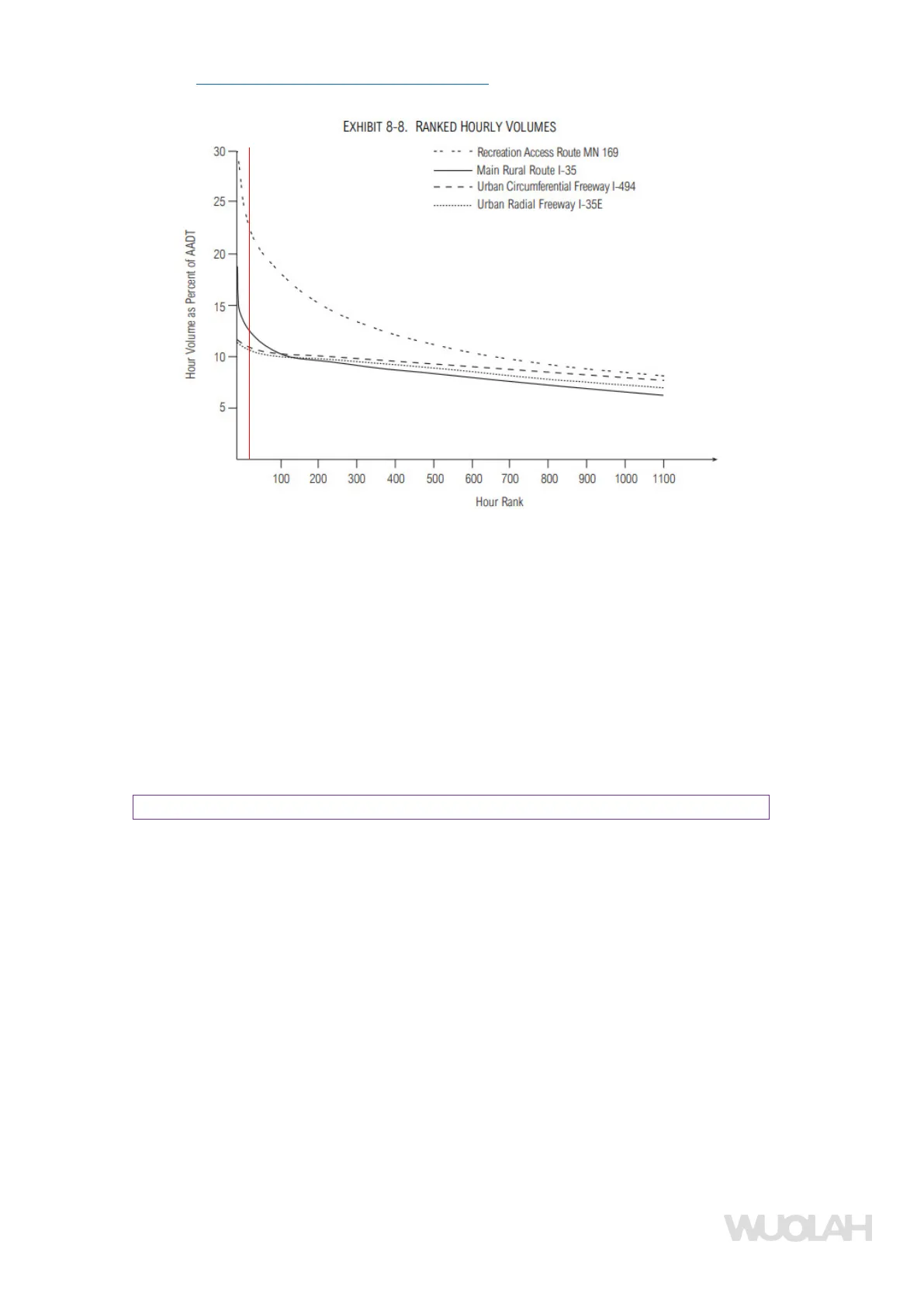
Design Hourly Volume (DHV): must guarantee good traffic conditions and at the same time guarantee that the road is not almost empty during most of the time. Empirically, its value corresponds to the 30th highest hourly traffic volume of the year. In most roads, DHV (30th highest hourly volume) is 11% - 17% of AADT (usually 13 - 14%). In touristic areas, it can go beyond 20%, while in arterials roads it can drop to 8%. See graph below:

WUOLAH Reservados todos los derechos. No se permite la explotación económica ni la transformación de esta obra. Queda permitida la impresión en su totalidad. #CanetRockCaprabo REGISTRA TU TICKET CANETROCK 022 CALLARIADaniel Plaza Herrera, Jonathan Sanz Carcelén More at: www.wuolah.com/profile/danielph147/uploaded

Ranked Hourly Volumes Exhibit

EXHIBIT 8-8. RANKED HOURLY VOLUMES 30 - Recreation Access Route MN 169 Main Rural Route 1-35 - Urban Circumferential Freeway 1-494 25- Urban Radial Freeway 1-35E Hour Volume as Percent of AADT 20 15- 10 5 100 200 300 400 500 600 700 800 900 1000 1100 Hour Rank Highway Capacity Manual 2000. Data from roads in Minnesota.

Velocity or Speed Factors

It is affected by flow, density, geometry, pavement, weather and geography.

• Time mean velocity (vt) (km/h) arithmetic average of the individual speeds of the cars passing a point in a road or lane.
• Space mean velocity (vs) (km/h). Two ways to compute it: a. Harmonic mean of speeds over a specific segment of road. b. Using the average travel time for vehicles to pass a segment of road.
• Average travel speed: the length of the segment divided by the average travel time of all vehicles traversing the segment (including stops and delays of cars). It's the most representative and the most difficult to measure (monitorised segments required).

Density Measurement

Number of vehicles per unit length. We can study the whole road, one direction or one lane. Can be computed taking a picture of a roadway section, but it is normally indirectly obtained from flow and speed. The higher the density, the lower the flow and the speed.

Other Traffic Variables

Mean time interval between vehicles, mean travel time, mean delay and continuous/discont flow.

Fundamental Relation of Traffic Flow

q = v . k Where q is flow, v is the space mean speed and k is density. Usually: vt = 1.02 . 05

2 WUOLAH si lees esto me debes un besito Reservados todos los derechos. No se permite la explotación económica ni la transformación de esta obra. Queda permitida la impresión en su totalidad.Daniel Plaza Herrera, Jonathan Sanz Carcelén More at: www.wuolah.com/profile/danielph147/uploaded

Generalized Relationships Among Speed, Density, and Flow Rate

EXHIBIT 7-2. GENERALIZED RELATIONSHIPS AMONG SPEED, DENSITY, AND FLOW RATE ON UNINTERRUPTED-FLOW FACILITIES Sf Sf Speed (km/h) So Speed (km/h) Do So - D 0 Do Dj 0 Vm Density (veh/km/In) Flow (veh/h/In) Sa Vm Sf Flow (veh/h/In) Legend Oversaturated flow -- 0 Do Di Density (veh/km/In) Nomenclature Sf Free-flow speed So Capacity speed Do kc Critical density Di ki Jam density Vm qmax Capacity (max flow)

Density-Speed Relationship

The critical density kc marks the point from where we change from a free to a congested flow. The jam density kj considers the whole lane filled with cars touching one another (v = 0). Usually: kc = (30 - 40%) · kj (not to scale in the graph). As we increase density, speed decreases.

Flow-Speed Relationship

We assume free-flow speed of which normally coincides with the speed limit. The maximum flow (qmax) is the capacity of the road. As we increase flow, speed decreases. Under congested flow, flow and speed reduce.

Density-Flow Relationship

The critical density kc marks the point from where we change from a free to a congested flow. The jam density kj considers the whole lane filled with cars touching one another (v = 0). Usually: kc = (30 - 40%) . kj (not to scale in the graph). As we increase density, flow increases. Under congested flow, if density grows, flow decreases.

3 WUOLAH si lees esto me debes un besito Reservados todos los derechos. No se permite la explotación económica ni la transformación de esta obra. Queda permitida la impresión en su totalidad.Daniel Plaza Herrera, Jonathan Sanz Carcelén More at: www.wuolah.com/profile/danielph147/uploaded

Traffic Analysis

Types of Traffic on New Roads

• Attracted traffic: coming from other roads.
• Induced traffic: a better road attracts new users.
• Generated traffic: a better road improves economy, generating new traffic.
• Converted traffic: conversion from another mode of transport.

Traffic Studies and Prognosis

Two types of traffic studies (capacity analysis): prognosis and on-site data collection. Shadow toll: administrations pay for the number of cars (mainly heavy vehicles) that use a road. Prognosis: we consider a linear annual growth. The Annual Average Daily Traffic in year n is: AADTn = AADTO . (1 + G)2 where G is the average annual growth.

On-Site Data Collection Methods

• Manual collection is very precise and differentiates between types of vehicles, but it has a high cost (salaries) and counting is limited in time.
• Rubber road tube is transversally placed in the road. Every time a car passes, the air inside is compressed and transmits a signal to a counter. It has low cost and measures speed, but it has a one-week life service and it cannot differentiate vehicle types.
• Inductive loop counter counts cars by the change in the electromagnetic field they produce. The variation in current is proportional to weight, so we can differentiate types of vehicles (motorbikes, cars, light trucks and heavy trucks). It also measures speed. The loop is embedded in the pavement and connected to a counter in the shoulder.

Roadway Network Capacity Analysis

Usually, when we build a road, we don't have a traffic study. For this reason, each year the administration designs a capacity analysis strategy for the roadway network.

Flow and Speed Measurement Methods

Four ways to measure flow and speed in roadways:

Permanent Traffic Gauging Stations

Permanent traffic gauging stations use inductive loop counters. They provide the AADT and the DHV with absolute precision. They also provide the seasonal, weekly, daily and hour variations of the AADT. These stations must be widespread in the network.

Primary Control Stations

Primary control stations are rubber road tubes. The AADT and the DHV is approximate. In most roads, DHV (30th highest hourly volume) is 11% - 17% of AADT (usually 13 - 14%).

• Option 1: 4 consecutive days (mandatory to include a weekend) every 2 months. This means we count 24 days per year. AADT 5 . ADTweekday + 2 . ADTweekend 7
• Option 2: 7 consecutive days every 2 months. This means, 42 days/yr (12 weekend days). AADT = = 1 Sunday · Monday ∑ ADTi

4 WUOLAH si lees esto me debes un besito Reservados todos los derechos. No se permite la explotación económica ni la transformación de esta obra. Queda permitida la impresión en su totalidad.caprabo te lleva gratis al CANETROCK 023 ESTRELLA 1 de Julio 4 Canet de Mar (Barcelona) Del 11 de mayo al 18 de junio, llévate una ENTRADA GRATIS* por una compra superior a 160 € Registra tu tiquet de compra en https://promociones. caprabo.com/es/ Además, si consigues tu entrada, participas en un SORTEO EXTRA de 3 pases dobles "Live Experience" para disfrutar en el propio escenario de tu grupo favorito. Daniel Plaza Herrera, Jonathan Sanz Carcelén More at: www.wuolah.com/profile/danielph147/uploaded

Traffic Factors from Stations

From these first two stations we can obtain other traffic factors:

• Nighttime factor (N): ratio between the Average Weekday Daily Traffic (AWDT) in a specific month and the AWDT computed for 16 hours (6 AM - 10 PM).
• Seasonal factor (L): ratio between the AWDT and its value in a specific month.
• Public holidays or weekend factor (S): ratio between AADT and AWDT.

AWDT N = AWDT 24h month AW DT16h month L = AW DT month S = AADT AW DT

Secondary Control Stations

Secondary control stations: manual or rubber tube counters. They don't obtain the previous factors.

• Option 1: 2 working days every 2 months (12 working days/yr).
• Option 2: 1 working day every 2 months (6 working days/yr).

We obtain the AADT using the public holiday factor: AADT = S . AWDT.

Coverage Control Stations

Coverage control stations: manual. They don't obtain the previous factors.

• Option 1: 1 working day per year. AADT = L . S . AWDT month
• Option 2: 16h (6 - 22h) of a working day per year. AADT = N . L . S . AWDT16h month

Capacity

Capacity Definition and Conditions

Capacity is the maximum number of vehicles that can go through a section of road during a period of time. It's a kind of flow. In order to reach capacity:

• traffic demand at the access of the road must be enough;
• the previous road section must have a higher capacity; and/or
• the next road section must have a higher capacity.

Level of Service Categories

Level of service (LOS), categories from A to F:

• A. Each user travels at his/her free speed. When a vehicle reaches another slower it can overtake without delay.
• B. The faster vehicles can overtake slower ones without delay. Most of users travel at their free speed.
• C. The faster vehicles must slow down to overtake slower ones. Most users cannot travel at their free speed.
• D. All users must reduce their speed because of preceding vehicles. The average speed is reduced.
• E. The average speed of all vehicles is practically the same and reduced. The traffic is like a train, with all the vehicles travelling at the same speed.
• F. All situations in which capacity is exceeded and there are traffic jams. Some vehicles must stop eventually.

Factors Affecting Capacity and LOS

• Road-related factors: number of lanes, lane width (only influences up to 3.6 m), distance to side obstacles / clearance (only up to 1.8 m), design speed and slopes.
• Traffic-related factors: heavy vehicles, traffic distribution among lanes, drivers experience (we will normally consider it as 1) and flow variations.
• Regulations: % of length where overtaking is allowed, speed limits.
• Meteorology: wind, fog rain ... Not taken into account for the computation of capacity.

WUOLAH Reservados todos los derechos. No se permite la explotación económica ni la transformación de esta obra. Queda permitida la impresión en su totalidad. #CanetRockCaprabo REGISTRA TU TICKET CANETROCK 022 CALLARIA