Costs and Profits in Microeconomics: Production Factors and Cost Curves

Costs and Profits Overview

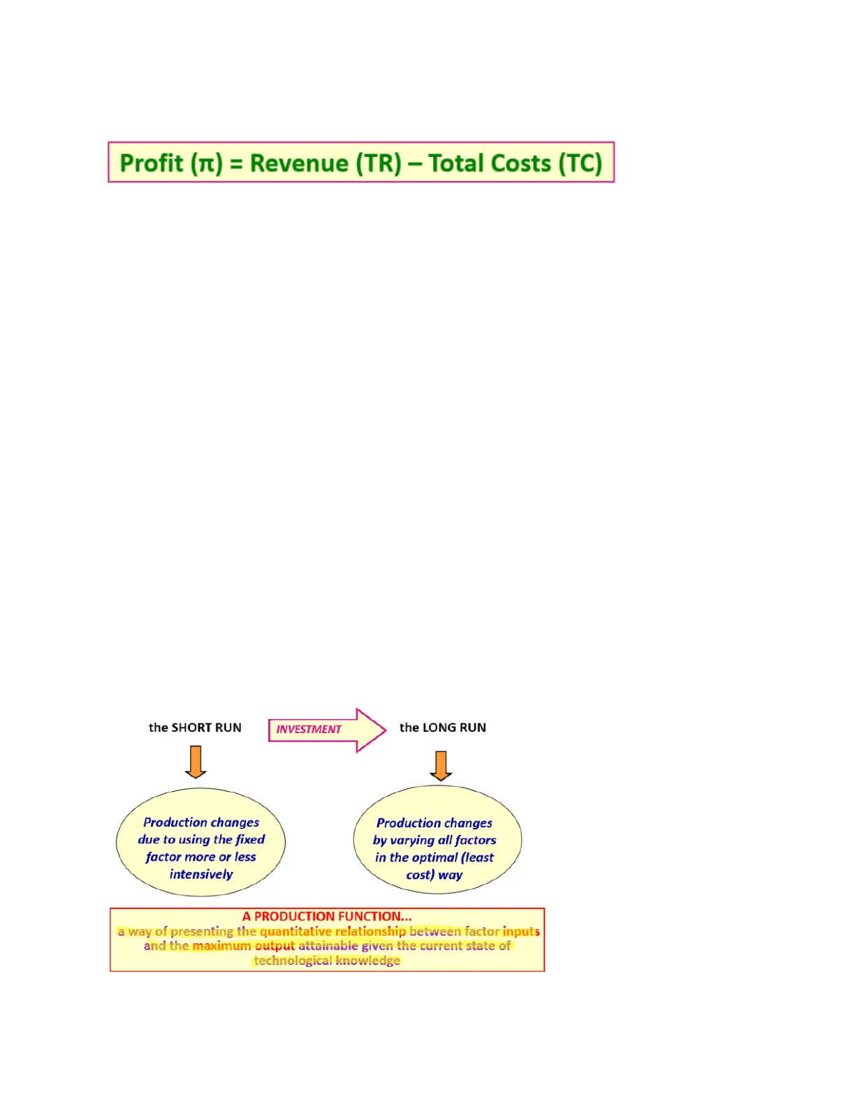
Profit (Tt) = Revenue (TR) - Total Costs (TC)
Costs helps a firm maximize its profitability in two ways:

• Technical efficiency: when a 'given' level of output is produced using the minimum
  amount of inputs (avoiding waste)
• 'optimal' level of production depends on both costs and market demand
  conditions

To understand the costs first the production process needs to be understood which is what
generates a firm's costs

Factors of Production and Time

A firm can produce goods and services by combining the Four Factors of Production

• Firms have choices as how they are combined
• Different combinations of factors willl have different costs associated with them

Short Run vs. Long Run

• The short run
  • Is the time of period over which a least one factor is fixed (often capital or land)
• The long run
  • Is the time period over which all factors are variable (no such thing as fixed
    factor of production)

the SHORT RUN
INVESTMENT
the LONG RUN
Production changes
due to using the fixed
factor more or less
intensively
Production changes
by varying all factors
in the optimal (least
cost) way

Production Function

A PRODUCTION FUNCTION ...
a way of presenting the quantitative relationship between factor inputs
and the maximum output attainable given the current state of
technological knowledge

Definitions of Product Measures

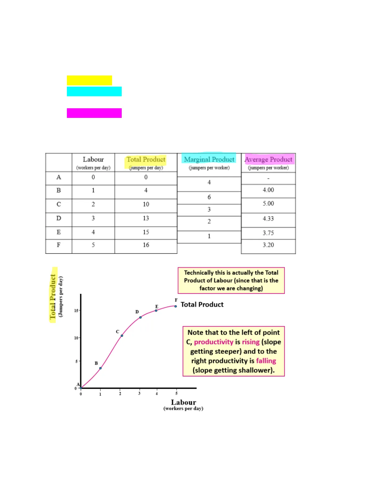
• Total product: the total amount produced
• Marginal product: the change in total product resulting from one unit-increase in a
  variable factor (in this case labour)
• Average product: of an input in the total product divided by the quantity of the input
  used
  • TOTAL PRODUCT / QUANTITY OF THE INPUT USED

Labour
(workers per day)
Total Product
(jumpers per day)
Marginal Product
(jumpers per worker)
Average Product
(jumpers per worker)
A
0
0
4
4.00
C
2
10
3
D
3
13
2
4.33
E
4
15
1
3.75
F
5
16
3.20

Total Product Curve Analysis

Total Product
(Jumpers per day)
Technically this is actually the Total
Product of Labour (since that is the
factor we are changing)
F
Total Product
E
15-
D
C
10-
5 -
B
Note that to the left of point
C, productivity is rising (slope
getting steeper) and to the
right productivity is falling
(slope getting shallower).
A
0
1
2
3
14
5
Labour
(workers per day)
-
B
1
4
6
5.00

Marginal Product Curve Analysis

Marginal Product
(Jumpers per person per day)
Note that Marginal Product is
also measured by the slope of
the Total Product curve
Technically this is actually
the Marginal Product of
Labour (since that is the
factor we are changing)
Marginal Product
0
Labour
(workers per day)

As a firm uses more of a variable input, with a given quantity of fixed inputs, there will come
a point when each additional unit of the variable factor will produce less extra output then
the previous unit.
This is what gives the MP curve its "bell" shape
Initially the MP of an additional worker exceeds the MP of the previous worker

• This occurs due to specialization/division of labour
• This is what we call increasing marginal return

At some point Diminishing Marginal returns sets in which is where the MP of an additional
worker is less than the MP of the previous worker

• More and more worrkers are using the same amount of machinery, so there is less
  for the additional workers to do

Law of Diminishing Returns

Marginal Product
(Jumpers per person per day
Law of Diminishing Returns sets in
Increasing Marginal Returns
Diminishing Marginal Returns
Marginal Product
0
Labour
(workers per day)

Average Product and Marginal Product Relationship

Average product
Marginal Product
(Jumpers per person per day)
In essence this behaves like any other average variable
Note that the MP curve always intersects
the AP curve at its highest point
Average Product
Marginal Product
Labour
(workers per day)

From Production to Costs

We describe the relationship between output and costs by using three concepts

• Total costs are the cost of all the factors of production the firm uses
• Marginal cost is the change in Total Cost from one unit-increases in output
• Average cost is the cost per unit of output

Short-Run Cost Analysis

The impact of short-run analysis
In the short run some inputs are fixed. Their costs are therefore fixed
Other inputs can be varied. Their costs are therefore variable.

• Total fixed cost is the cost of fixed inputs
• Total variable cost is the cost of variable inputs
• Total cost is the sum of both
  TC = TFC +TVC

If we assume capital costs are £25, and it costs £25 to employ
a unit of labour, we can construct the following:

Labour
(workers per day)
Output
(jumpers per day)
TFC
(£ per day)
TVC
(£ per day)
TC
(£ per day)
0
0
25
0
25
1
4
25
25
50
2
10
25
50
75
3
13
25
75
100
4
15
25
100
125
5
16
25
125
150

Total Cost Curve

(pounds per day)
TC
Cost
TVC
1
TFC
İ
0
0
Output
(jumpers per day)

Average and Marginal Costs

Average cost and marginal costs

• Average cost is the cost per unit of production
  • Average fixed cost
  • Average variable cost
  • Average total cost
    TC = TFC + TVC
    Q
    Q
• Marginal cost is the total cost of production one extra unit of output:
  MC = ATC / AQ

Marginal Cost and Average Cost Curves

MARGINAL COST AND AVERAGE COSTS
Costs (£)
MC
ATC
Note minimum points
for ATC & AVC, and
their intersection with
AVC
MC curve!
1
1
AFC
Output (Q)

• Marginal cost and ATC are 'U-shaped' because initially there are economies due to
  specialization but ultimately the diminishing returns arrive
• The AVC curve gets closer and closer to ATC because FC are being spread over
  increasing amounts of output

Long Run Cost Analysis

The long run

• All factors of production are variable
• The object is to minisme production costs for a given amount of output
• The main focus is upon altering the size of the capital stock to achieve the least cost
  means of production
  • Just as we had diminishing returns to labour, we also have diminishing returns to
    capital (when labour is fixed)
  • Need to find the optimal blend of the factor of production

Optimal Factory Size

FROM PRODUCTION TO COSTS
Costs (£)
What is the Optimal factory size?
If Output 0-Q1, then Factory 1
If Output is Q1-Q2, then Factory 2
If Output is > Q2, then Factory 3
SRATC2
SRATC1
SRATC3
With larger factories,
there are higher fixed
costs thus SRATC are
minimised at higher levels
of output
0
Q1
Q2
Quantity (Q)

Short Run to Long Run Average Cost

FROM SR TO LR
Costs (£)
AC in the Long Run is made up from
a 'family' of SR-ATC curves!
SRATC2
SRATC3
SRATC1
LRAC
0
Quantity (Q)

Theoretically there are an infinite number of factory sizes
Costs (£)
SRATC
SRATC
SRATC
SRATC
SRATC
LRAC
0
Quantity (Q)

• The long run is just a series of short runs as every short run cost can be turned into
  long run
• The LRAC provides a description of the lowest cost method of producing any given
  amount of output
• SRATC curves are tangential to LRAC curve

Why LR-AC is U-Shaped

WHY IS LR-AC 'U' SHAPED?
Costs (£)
Increasing Returns to Scale LRAC V
Constant Returns to Scale LRAC-
Decreasing Returns to Scale LRACÎ
IRS
CRS
DRS
LRAC
Economies of
Scale
Diseconomies of Scale
0
Minimum Efficient
Scale (MES)
Quantity (Q)

Economies and Diseconomies of Scale

Economies of scale and diseconomies of scale

• Economies of scale are feature of a firms technology that lead to falling long run
  average cost as production increases
  • Specialization of labour and capital
  • Bulk buying
  • Indivisibility
  • Greater efficiency of large machines
  • The container principle
  • Organizational efficiencies
  • Finanancial economies
  • Economies of scope (variety not volume)
  • External economies
• Diseconomies of scale are the features of a firm's technology that lead to rising
  long run average cost as production increases
  • Complex management and organization structures