Regression and supervised learning algorithms: Ridge and Lasso

REGRESSION

SUPERVISED LEARNING

It is a setting in which data from an unknown function map an input x to an output t: D = {{x, t)}. Input variables x are usually called features or attributes, output variables t are also called targets or labels. The goal is to find the best possible approximation of f, the mapping function. The function f does not need to be deterministic, it can have statistical uncertainty. Two assumptions that need to be made are that the relationship f is existing for data in the domain D, and that the function must be repeatable over the same dataset in time.

Depending on the nature of t, there will be different forms of supervised learning:

• If t is a continuous variable, the technique of choice will be regression
• If t is a discrete variable, the technique of choice will be classification
• If t is a model of being a probability of belonging to a group, the technique of choice will be a mix between regression and classification (technically, a peculiar classification)

STEPWISE APPROACH

If we imagine of drawing a set F of all the possible functions that go from the input space to the target space, we can assume that there exists only one function f being the best one to approximate. In any problem, we define an input, a target, and a domain of (usually infinite) functions mapping the input into the target. Supervised learning tries to solve an optimization problem, thus approximating a function f given the dataset D.

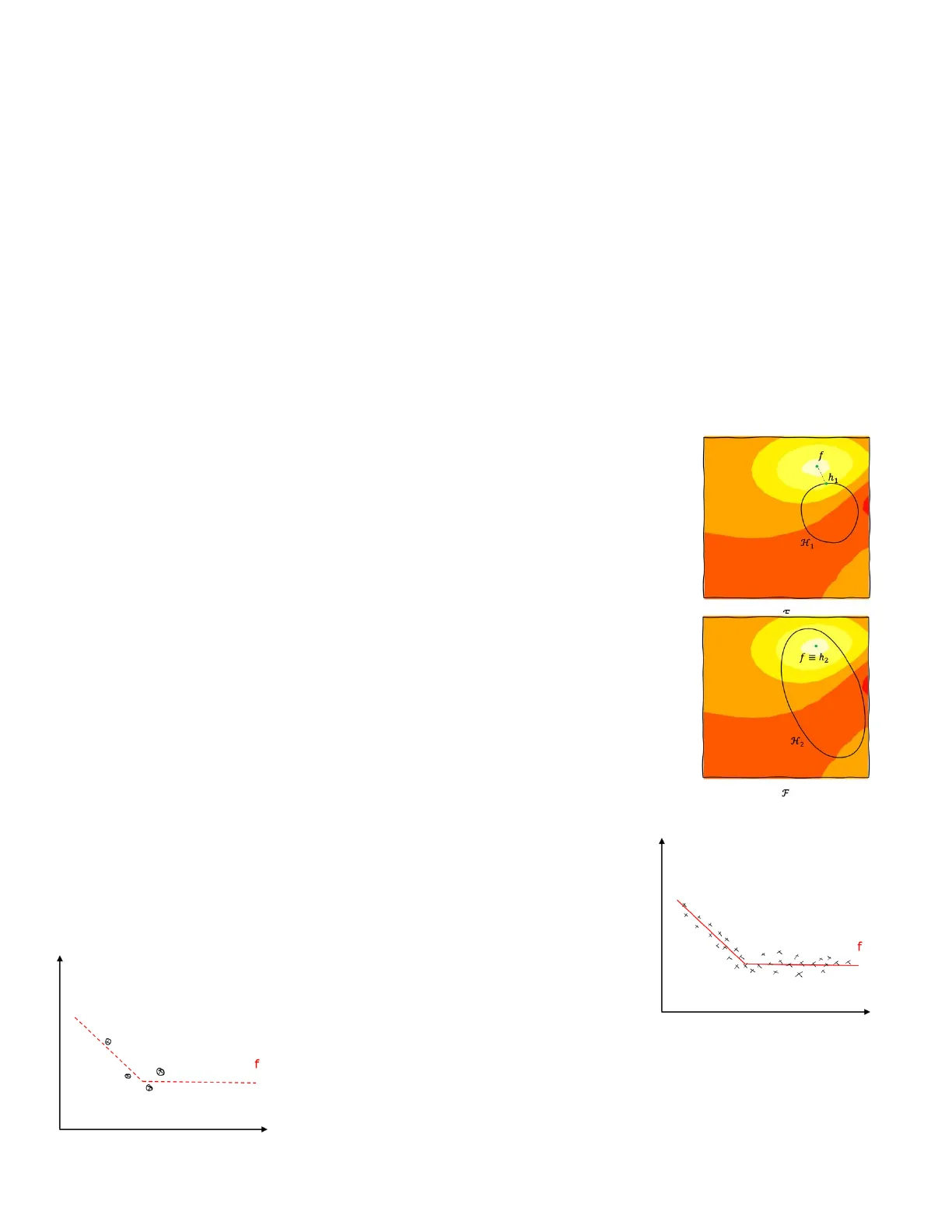
• The first step is the definition of the loss function L: write a numerical evaluation that tells how far any approximation in the space F (of all the possible functions) you can find as approximation of f. The lighter the color, the less is the loss, the better is the approximation, meaning that the approximation function is close to the actual one (f).
• The second step is to define a family of models of the approximation function, called hypothesis space H.
• The last step is the optimization algorithm that is able to optimize the loss inside the hypothesis space.

When defining the hypothesis space, we cannot be sure that it will contain the optimal approximation. h1 is the best approximation in the example in the hypothesis space H (}{II). If the family of functions H, chosen to find an approximation, is larger, then we can hope to have a larger hypothesis space containing the true function f to approximate. If the optimization process is good enough, we will be able to find exactly the mapping function f. Indeed, this is not always the case.

f h1 H f = h2 H2

The true problem of supervised learning is that f is unknown, therefore it is almost F impossible to end up having a "nice" loss function as in the image. This is the key problem of supervised learning, the most important concept behind machine learning.

Example

Let's consider the true function f generating the data in the image. (>)

The true function is given by the red line + some noise, so it can be represented as follows (4)

f × f

What can be considered when trying to approximate the red line are just some data points (the circles are 4 data points).

1If we choose a family of linear approximation functions (very easy), the best thing we can learn is something like in the image, which is very different from the original function f.

The real problem when having just these four points is that we have no clue on how to compute the approximation function h1. That's because we have no way of understanding how far h1 is from f in other regions of the hypothesis space, where we have no points. Hence, we cannot improve our approximation function.

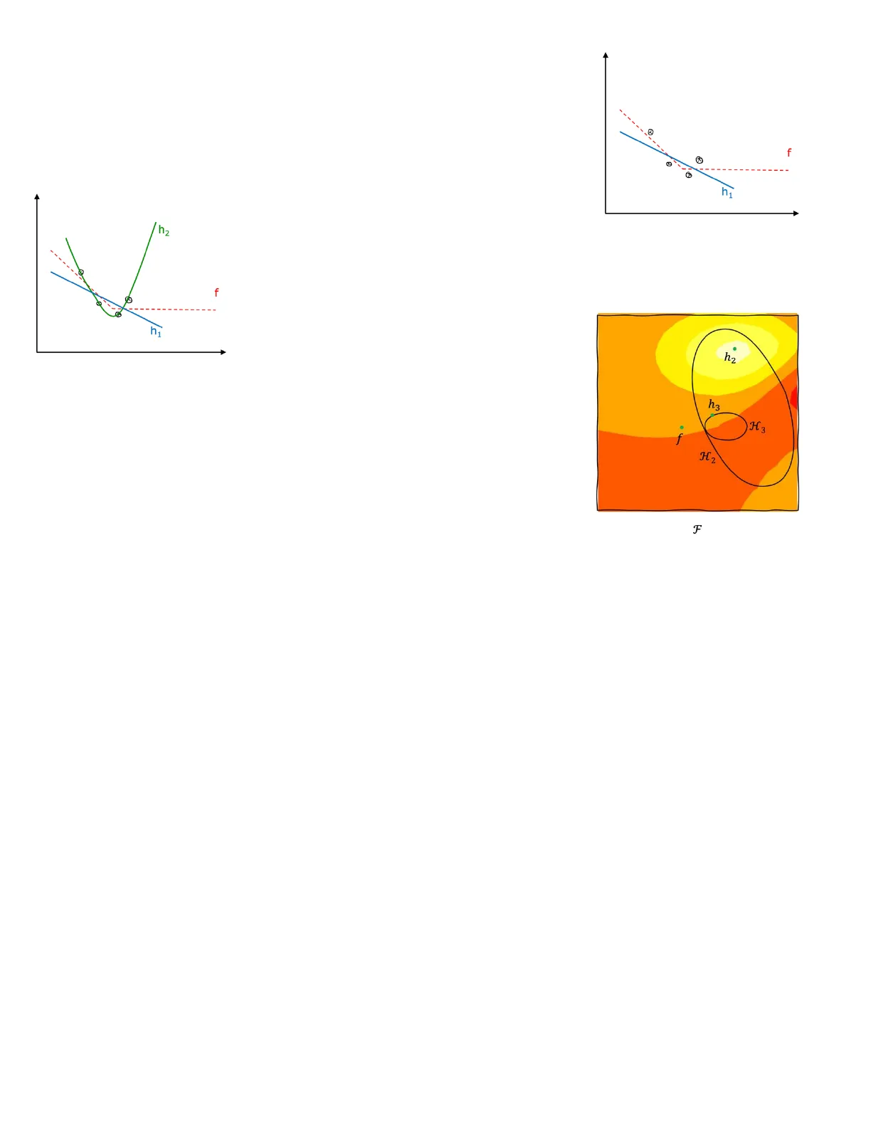
h2 f h h2 does not correspond to the optimal value of the loss function. Sometimes, a restriction in the hypothesis space can lead to better solutions as larger mistakes can be avoided thanks to that restriction.

ELEMENTS OF SUPERVISED LEARNING ALGORITHMS

• Representation
• Evaluation
• Optimization

-- f 0 h1

We can increase the size of the hypothesis space, moving to a quadratic model. We obtain h2. From the point of view of the 4 known points, this curve seems perfectly fit, however by comparing the errors we make with respect to the true function, the error made by h1 is better with respect to the red line.

h2 h3 H3 f H2 F

LINEAR REGRESSION

Linear regression model is not as limiting as it may appear and is not used only in the simplest cases.

In the regression problem, we have some data consisting of input variables (e.g., x) and a target variable (e.g., y). The aim is to find a model to predict the value of the target variable based on the input variables.

In the simple setting reported (->), the easiest way to predict the variable y is the average of y itself. We use basic average as a predictor. It is a very simple baseline, but it represents the simplest possible model and a value to evaluate other models. Since it is the baseline, we expect that all other models are better.

SIMPLE LINEAR MODEL

Simple linear model is basically a line that try to minimize the errors while fitting all the data points. Note that we are not only training the red line to find the relationship between x and y, but also to apply this model on a new set of data point. It is likely that on the new set of data, the model we'll make some mistakes. Still, the aim of training is to minimize such error when we apply the model to different datasets.

MODEL, LOSS, AND OPTIMIZATION

Model

• The simplest linear model can be defined as y (target) being the sum between a constant weight W0 (called bias parameter, it represents the intercept with y axis) and the input variables multiplied by a weight (e.g., W1). y = Wo + W1X o Recalling the hypothesis space (the ellipsis where all possible models can lie), in this case the hypothesis space is represented by all the possible combinations of W0 and W1 (upper plot). o Each possible combination (blue dots in the upper plot) represents a red line (possible model).
• For each point Xi in the dataset, the prediction will be based on weights and will give an output Yi. The error made will be the difference between the true value of the target variable (Ti) and the predicted Yi. yi = Wo + W1Xi Ei = ti - yi o Note that Ei is the prediction error, also called residual.

125 100 75 50 25 0 -25 -50 0 2 * The training data points 125 100 75 50 25 0 -25 -50 -2 -1 1 2 M y=34.574x+53.176 125 100 75 50 25 0 -25 -50 -2 -1 0 1 2 x W1 Wo 7 x

Loss

We need to quantify in an objective way the error made in order to minimize it. In general, mistakes are represented with loss functions. The most convenient is the residual sum of squares.

• The residual sum of squares (RSS) or the sum of squared errors (SSE) is the sum of all the residuals squared.
• The squaring is made in order to get only positive values, otherwise the overall sum of residuals will be small since there are some negative errors (overestimation).
• Thanks to the RSS, we can now assign to each point in the WO-W1 space a loss value. In the end, we will take the point in space with the lowest loss value.

RSS(wo,W1)=>€ ?= >(ti-(wo+w1X1)2 i=1 N i=1 N L = 2.8 . 105 · L = 3.3 . 105 ·- L = 7.6 . 103 W1 · L = 5.4.104 L = 1.0 . 105 L = 1.0 . 106 . wo 7 X

Optimization

From a mathematical perspective, the RSS is a quadratic loss function. Thus, in order to find the optimum value of W0 and W1 we look for a minimum in the equation. Indeed, we compute the derivative with respect to each weight.

VRSS(wo, w1)= -2Ei-1 (ti-(wo + w1;) -2 Ei-1 (ti- (wo + wifi) Ti RSS

4* W Since it is a multivariate function (depends on both w0 and w1), the derivative procedure will give us two functions. It is called gradient and corresponds to the vector containing all the partial derivatives of a function. Then, we have two possible approaches:

• Approach 1 (Ordinary Least Squares - OLS) o Set the gradient of the RSS(W0, W1) to zero Might be unfeasible from a computational point of view if we have a very large number of points (variables). o
• Approach 2 (Gradient descent) o Apply gradient descent until convergence: n+1 W = wn - aVRSS(wn2) It is more computational convenient approach. o The idea is to not look for the value of W where the gradient is zero, but to update over and over the weight vector in the direction of the gradient. This way, we slowly reach the bottom. o It is even more convenient when we perform a stochastic gradient descent. Instead of computing the gradient on all points, we compute it just on a smaller number of point. o If a is large, we are making large steps but might not converge. If a is small, we might be very slow. Thus, a rule of thumb to set a is to make it adapt over time, e.g., a" = aº/n or a" = aº/Vn. Note that the value of aº is chosen as trial and error.

VRSS RSS Initial weight -- w* W

CAN WE GENERALIZE THE MODEL?

The simplest linear model can be defined to expand its dimensional space. We use the same approach as before having D variables. The first of all variables is equal to 1, thus in the input vector we will have 1 followed by D-1 variables. This is because the final model is the scalar product of our input variable vector and weights. Since the first weight W0 is a baseline, we multiply it by 1 (the first of all variables) in order to not change its value.

y(x, w) =w0+ D-1 j=1 > wjaj = wTx x=(1,x1, ... ,xp-1) Wo is the bias parameter associated with dummy variable 1 . Note that the T above the w means transposed: transposition is necessary for the scalar product (it must be a row multiplied by a column product).

CAN WE GENERALIZE THE MODEL EVEN MORE?

Even though we can generalize for multiple variables, we still have the problem of linearity. The model showed before is constrained in linearity, thus higher order relationship cannot be well approximated.

A linear combination of the input variables is not enough to model data, however we don't need input variables to be linear as far as a regression model that is linear in the parameters. Indeed, we can increase the order of the input variables, but we can still have a scalar product between weights and input. To increase the order, we are applying to the input vector a feature mapping ¢.

• A feature mapping + is any non-linear function. It is called feature mapping as we are applying a transformation to our input data to get a new set of data, called features.
• After the transformation with the feature mapping, rather that the scalar product between weight and input vector, we talk about of scalar product between weight and feature vector.
• The model will be still linear with respect to weight vector and feature but won't be linear with respect to the input space.
• Note that the dimension M of the feature vector is not necessarily the same of the dimension D of the input vector.

We can define a model using non-linear basis functions: y(x, w) = w0+ E j=1 M-1 wjØj(x)=w™¢(x) +(x)=(1,01(x), ... ,¢M-1(x))7

Example

In this case, we are adding a new variable called x2, the feature coming from the square of the variable x. If we combine the two variables, we can identify a new linear model using x and x2 in a higher dimensional space (from 1D to 2D). Note that the new variable may be more significant than the original one, thus in the end we will may end up with a feature space of the same of dimension of the input space or maybe both variables are significant and the dimensional space is higher. In the end, the solution in the original input space will appear as in the yellow balloon.

2 x 7 X X t . 7 x x2 x2