Programación matemática con restricciones de desigualdad, Universidad de Sevilla

Unit 5. Mathematical Programming with inequality constraints

Mathematics II Grado de Administración y Dirección de Empresas.

• 1. The Kuhn-Tucker necessary conditions.
• 2. Sufficient optimality conditions.Optimization with inequality constraints. The Kuhn-Tucker necessary conditions.

Consideraciones iniciales

Consider: Opt f(x) s.t. gj(x)≤bj, j=1, ... ,m where f : D C IR" -> IR, gj : R" -> R, j = 1, ... , m, f, g; have continuous partial derivatives. The set of feasible solutions X = {x € D : gj(x) ≤ bj, j = 1, ... , m}.

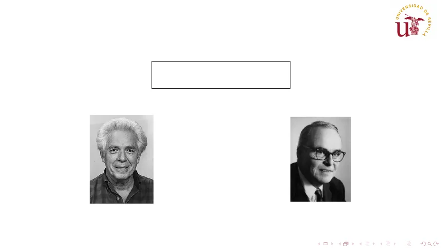
Harold W. Kuhn (1925-2014) Albert W. Tucker (1905-1995)

Optimization with inequality constraints

The feasible sets contain both interior and boundary points. The constraint gj(x) { bj is active at x* € X, if gj(x*) = bj. x* E X is in the boundary of X if and only if at least one of the constraints is active at x* . A point x* E X is interior if and only if no constraint is active at x ∗ . 9 x-y2=1 (2,1) xix (2, 1/2) AX (1,0) (3h, 1/2) x=2 X = {x - y2 ≥ 1, x < 2, y > 0} Two constraints are active at (2,1) and at (1,0), One constraint is active at (2, 1/2). No constraint is active at (3/2, 1/2). It is an interior point.

The Kuhn-Tucker necessary conditions

Opt f (x) s.t. gj(x)≤bj, j=1, ... ,m L(x; X) = f(x) ->\;(gj(x) - bj) m j=1 For x* E X, denote /(x*) = {j € {1, ... , m} : gj(x*) = bj} (the active constraints at x*). Assume that Vg(x*) for j E I(x*) are linearly independent. The Kuhn-Tucker necessary conditions for local optimality x* E X is a local maximum (minimum) => >* 2 0(< 0) exists, such that 1. VxC(x *; )*) = 0. 2. X*(gj(x*) - bj) = 0, Vj=1, ... , m. Condition 1 states that the derivates of the Lagrangian function with respect to the decision variables must be zero. Conditions 2 are called complementary slackness conditions. They state that at a local optimum, either a constraint is active or the corresponding multiplier is zero (or both). The interpretation of the multipliers coincides with that of the Lagrange multipliers.

Kuhn-Tucker conditions for maximization/minimization

Opt f(x) s.t. gj(x)≤bj, j=1, ... ,m m £(x; X) = f(x) ->\;(gj(x) - bj) j=1 (x*, *) is a Kuhn-Tucker(K-T) point for a maximization (minimization) problem: 1. VxC(x *; )*) = 0 > 2 (x*, *) = 0 for all i = 1, ... , n. 0xi 2. X*(gj(x*) - bj) = 0 for all j=1, ... , m. 3. , 2 0, for all j = 1,., m (); < 0, for all j = 1, ... , m). 4. gj(x*) ≤ bj for all j =1, ... , m.

Example 2: Max x^2 + y^2

Max x2 + y2 s.t. -x+y2≤-1 x≤ 2 [(x, y; ), M) =x2 + y2 - X(-x + y2 +1) - (x - 2). A Kuhn-Tucker point must fulfil: 1. 2x+ X - p=0 2y -2Xy = 0. 2. x(-x + y2 + 1) = 0 p(x-2)=0. 3. > > 0, u > 0. 4. - x+ y2 ≤ -1 × ≤ 2. To obtain the K-T points we start with the system of equations: 2×+X-p=0 2y - 2Xy = 0. X(-x+y2+1) = 0 p(x-2)=0. We obtain: (0,0;0,0), (2,0;0,4), (1,0; - 2,0), (2,1;1,5), (2,-1; 1,5). From among these points, those that fulfil the inequalities are: (2, 0; 0, 4), (2, 1; 1, 5), (2, -1; 1, 5). These are the K-T points. Is this sufficient to solve the problem?

Example 2: Weierstrass theorem application

Max ×2 + y2 s.t. -x+y2 ≤-1 x≤2 (2,2) x-y=1 (2,0) , (21-1) x=2 The Kuhn-Tucker necessary conditions are sufficent in this case to solve the problem, since the hypotheses of the Weierstrass theorem hold: the objective function, f(x, y) = x2 + y2 is continuous (it is a polynomial function). the feasible set is closed since it is described by <- constraints. Therefore, it contains its boundary. the feasible set is bounded: y2 < x - 1 < 2 - 1 = 1, therefore, -1 < y < 1. On the other hand, x ≥ y2 +1, and, therefore, 1 < x < 2. Alternatively, the boundedness of X can be explained as being due to X C E((0,0), 2). It follows that a global maximum (and a global minimum) exists. The maxima must be among those points fulfilling the Kuhn-Tucker conditions. By comparing the values attained by the objective functions, we obtain: f (2,0) =4, f(2,1) =5, f(2,-1) = 5. We conclude that (2,1) and (2,-1) are the global maxima.

Example 2: Min x^2 + y^2

Min x2 + y2 s.t. -x+y2 ≤-1 x≤2 (2,1) x-y=1 (2,0) (21-1) xx=2 The existence of a global minimum is guaranteed (Weierstrass theorem). The global minima fulfil the Kuhn-Tucker conditions for a minimization problem. K-T points: 1. 2x+X - p=0 2y -2Xy = 0. 2. X(-x+y2 + 1) = 0 p(x-2)=0. 3. 4. - x+y2 ≤ -1 x ≤ 2. The system of equations: 2x+1 -p=0 2y -2y = 0. X(-x+y2 + 1) = 0 p(x-2)=0. We obtain: (0,0;0,0), (2,0;0,4), (1,0; - 2,0), (2,1;1,5), (2,-1; 1,5). From among these points, only (1,0; - 2, 0) fulfils the inequalities, and therefore, it is the only Kuhn-Tucker point. As a conclusion: (1,0) is the global minimum.

Sufficient condition for global optimality

Opt f (x) s.t. gj(x)≤bj, j=1, ... ,m X = {x E D : g (x) ≤ bj, j =1, ... , m}. Sufficient condition for global optimality Let X C IR" be a convex set, and f convex (concave) in X (x *; )*) is a Kuhn-Tucker point => x* is a global minimum (maximum) of f in X. Moreover, if f is strictly convex (concave) in X, then the global minimum (maximum), if it exists, is unique.

Example 3: Min x^2 + y^2 (unbounded feasible set)

Min x2 + y2 s.t. -x+y2 ≤-1 4 Since the feasible set is not bounded, the existence of global optima is not guaranteed in advance. We analyse the convexity of the feasible set and of the objective function: f(x, y) = x2 + y2 is strictly convex in IR2 (previously shown). the feasible set: X = {(x, y) E IR2 : - x + y2 < - 1}. Note that X is a level set N(-1) for the function g(x, y) =- x+y2. We study its convexity. Vg(x, y) = ( 2) 2y Hg(x, y) = 0 0 0 2 This matrix is PSD in IR2. Therefore, g is convex and the level set N(-1) = X, is a convex set. , . System of equations: K-T points: 1. 2x + ) = 0 2y -2Xy = 0 2. X(-x+ y2 + 1) = 0 3. 150 4. - x+y2 ≤-1 2x + )=0 2y -2Xy = 0 X(-x+y2+1) = 0 We obtain: (0,0;0) and (1,0; - 2). However, only (1,0; - 2) is a K-T point. It follows from the sufficient condition that (1,0) is the global minimum. 5

The Kuhn-Tucker conditions with non-negative variables

Opt f(x) s.t. gj(x)≤bj, j=1, ... ,m x ≥ 0 j=1 m £(x; X) = f (x) - Aj(gj(x) - bj) (x*, )*) is a Kuhn-Tucker point for a maximization (minimization) problem: 1. VxC(x *; )*) ≤ 0 (VxC(x *; )*) ≥ 0). 2. xi * (x*, *) = 0 for all i =1, ... , n. axi 3. x* ≥ 0 for all i = 1, ... , n. 4. X(gj(x*) - bj) = 0 for all j=1, ... , m. 5. 1, 2 0, for all j = 1, ... , m (x < 0, for all j = 1, ., m). 6. gj(x*) { bj for all j = 1, ... , m.

Example 4: Max x+y with non-negative variables

Max x+y s.t. 2 + y ≤ 1 x, y ≥0 [(x, y; ) = x + y - x(x2 + y - 1). K-T points for maximization: 1. 1-2Xx≤0 1 -X≤0. 2. x(1- 2Xx) = 0 y(1-X)=0 3. x, y ≥ 0 4. X ≥ 0. 5. X(x2 + y - 1) = 0 6. x2 + y ≤ 1 System of equations: x(1-2\x) = 0 y(1 -X)=0. X(x2 + y - 1) = 0 We obtain: (0,0;0,), (1,0; 1/2), (-1,0 ;- 1/2), (0,1;1), (1/2,3/4;1). There is only one K-T point: (1/2,3/4;1). Is (1/2, 3/4) a global maximum?

Kuhn-Tucker conditions with non-negative variables: Convexity analysis

Max x+y s.t. x2+y ≤1 x, y ≥0 To study whether (1/2, 3/4) is the global maximum, in this case, two possibilities exist: a) Analyzing convexity: The objective function is linear, and therefore, it is concave. The feasible set is the intersection of two half-spaces, x ≥ 0,y ≥ 0 (which are convex sets) and of the set S = {(x, y) E IR2 : x2 + y ≤ 1}. S is the level set N1 of the function g(x, y) = x2 + y. g is convex in IR2 since Hg(x, y) = ( 2 0 is PSD in 0 0 IR2. Therefore, S is a convex set. The feasible set is convex since it is the intersection of three convex sets. It follows from the sufficient condition that, since (1/2, 3/4; 1) is a K-T point, then the point (1/2, 3/4) is the global maximum. (12 3 /4 ) (10) x+y= k.

Kuhn-Tucker conditions with non-negative variables: Weierstrass theorem

Max x+y s.t. x2 + y ≤1 x, y ≥0 To study whether (1/2, 3/4) is the global maximum, two possibilities exist: b) The Weierstrass theorem: The objective function is continuous since it is a linear function. The feasible set is closed since it contains its boundary. The feasible set is bounded: 0 < x ≤ 1, 0 ≤ y ≤ 1. (or, for instance, X CE((0,0),2)). Therefore, a global maximum exists. Since (1/2, 3/4; 1) is the only point fulfilling the Kuhn-Tucker necessary conditions, then (1/2, 3/4) is the global maximum. (1/2 , 3/ 4) 1 (10) x+y=K.

Kuhn-Tucker conditions with only some non-negative variables

Opt f(x) s.t. gj(x) ≤ bj, j=1, ... ,m xi ≥ 0,iET m £(x;X) = f(x)->\;(gj(x)-bj) j=1 If i ¢ T, then xi is unrestricted in sign (free). (x*, )*) is a K-T point for a maximization (minimization) problem: 1. *, *) ≤0 ( (*, *) ≥ 0), 1. (x*, *) = 0, for all i ¢ T. 2. Xi * axi (x*, *) = 0 for all i € T. 3. x* ≥ 0, for all i € T. 4. X;(gj(x*) - bj) = 0 for all j=1, ... , m. 5. * > 0, for all j = 1, ... , m (X); < 0, for all j = 1, . , m). 6. gj(x*) ≤ bj for all j =1, ... , m.

Example 5: Max x+y with some non-negative variables

Opt x+y s.t. x2 + y ≤1 × ≥ 0 [(x, y; ) = x + y - X(x2 + y - 1). K-T conditions for maxima: 1. 1-2Xx≤0 1 - )=0 2. x(1- 2)x) = 0 3. x ≥ 0 4. X > 0 5. X(×2 + y - 1) = 0 6. x2 + y ≤ 1 System of equations: 1 - X=0 x(1-2)x) = 0 X(×2 + y - 1) = 0 We obtain: (0,1; 1) and (1/2,3/4; 1). The only K-T point is (1/2,3/4;1). Similarly as in the previous example, the sufficient condition permits us to conclude that (1/2, 3/4) is the only global maximum.

Kuhn-Tucker conditions with only some non-negative variables: Minima

Opt x+y s.t. x2 + y < 1 x≥0 C(x,y; ) = x + y - x(x2 + y - 1). K-T conditions for minima: From the system of equations: (0,1;1), (1/2,3/4;1). None of them is a K-T point, therefore no K-T point exists and no minimum exists. 1. 1-2Xx >0 1- >=0 2. x(1-2\x) = 0 3. x ≥ 0 4. >< 0 5. X(×2 + y - 1) = 0 6. x2 + y ≤ 1 Max 2

Problems with only non-negativity constraints

Opt f ( x) s.t. x ≥ 0 Necessary conditions for local optimality x* is a local maximum (minimum) => 1. Vf(x*) ≤0(Vf(x*) ≥0) of of (x*) ≤0((x*) ≥ 0) for i=1, ... , n. Of 2. Xi aXi * (x*) = 0 for i =1, ... , n. 3. x* > 0 for i = 1, . . . , n.