Statistical Inference: Central Limit Theorem and Confidence Intervals

Statistical Inference

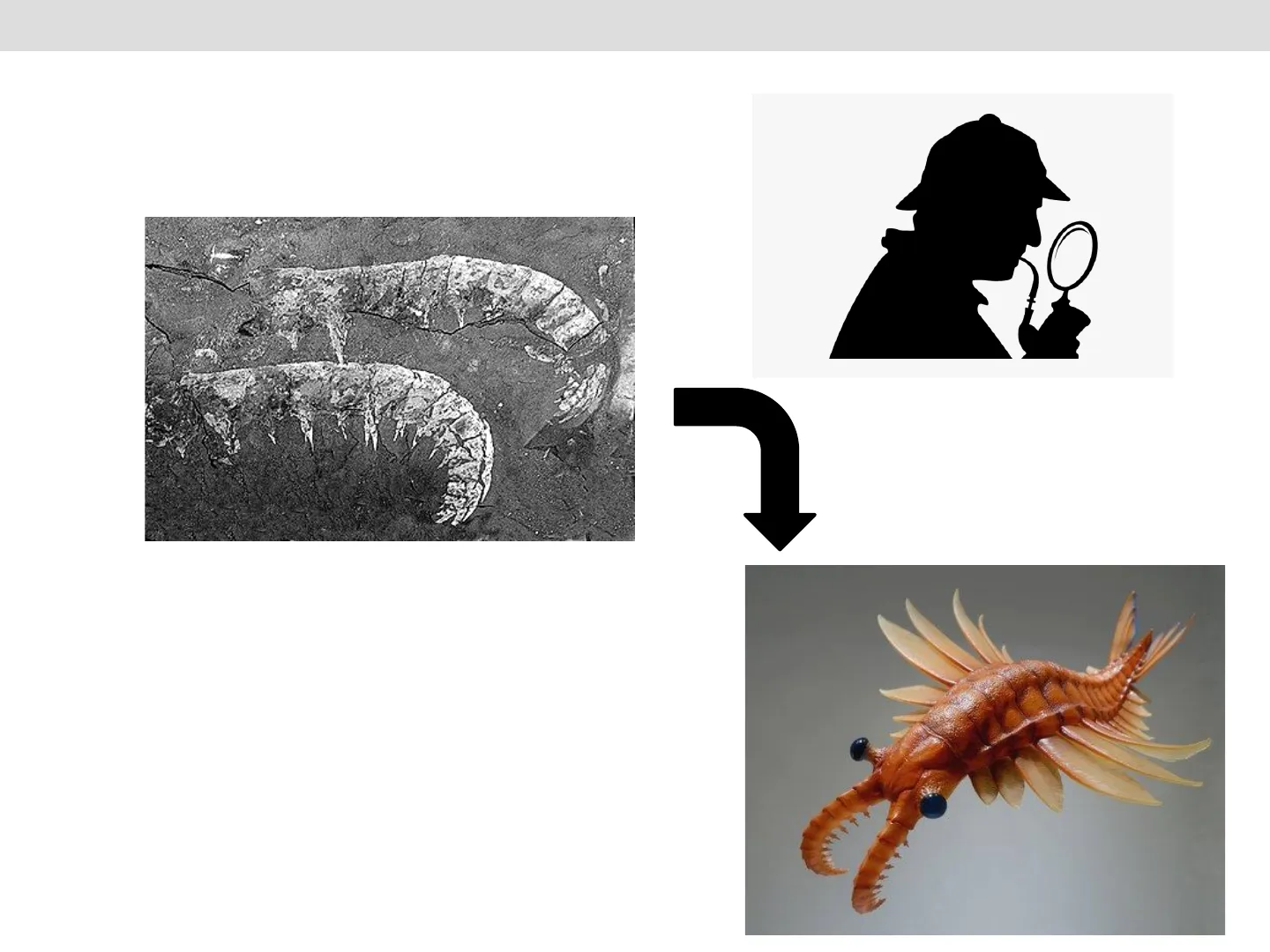
Image: Fossil and reconstruction of Anomalocaris canadiensis

Branches of Statistics

• DESCRIPTIVE
• POPULATION
• MEAN
• VARIANCE

• Parameters
• DESCRIPTIVE
• SAMPLE
• MEAN
• VARIANCE
• INFERENTIAL

Key Ideas in Parameter Estimation

• A sample of individuals is observed. The results of interest are generalized to the population where the sample was taken (Statistical Inference).
• If the sample is not representative of the population the results of inference are incorrect.
• Although the sample is representative, the results obtained in the sample will not coincide with those of the population. This is due to the variability of random samples.
• The uncertainty of the results of a sample depends greatly on the size of the sample. Small samples produce more uncertain estimates than large samples.

Example of Parameter Estimation

• We select a sample to study a variable X, for example body mass index (BMI)
• We want to know the BMI mean
• We compute the sample mean: (mean BMI of 15 people)
• We would like to use it as an estimate of the population mean

XBMI estimator

PBMI parameter

Question:

• Is the sample mean a good enough estimator of the population mean?

Considerations for Estimation

• Probably it is better to know the BMI mean of a sample than to know nothing
• But we need to evaluate the degree of uncertainty associated with our estimate

That means:

• If the study was repeated using a similar sample, what value would BMI have?
• One way of addressing this problem is to assume that we can extract many samples with same size from the original population
• What can be said of the samples' means in relation to the population mean?

Sampling Distribution

Population Die Rolls

Population: 2500 die rolls ( mean= 3.52 )

400 300 Count 200 100 - 0 1 2 -m 4 5 6 dice

Samples N = 2 (mean of two dice)

Sample 1 -- > 4.0 Sample 2 -- > 2.0 Sample 3 -- > 6.0 Sample 4 -- > 3.0 Sample 5 -- > 3.5 Sample 6 -- > 3.0 Sample 7 -- > 6.0 . ..

• Each experiment gives a different result.
• Sometimes very wrong!
• If we could repeat the experiment many times, we would get a distribution of the sampling results. This is called a sampling distribution.

mean of means = 3.523

Sampling Distribution of Means

Population: 2500 die rolls ( mean= 3.52 )

400 300 Count 200 100 - 0 1 2 -m 4 5 6 dice

Samples N = 2 (mean of two dice)

Sample 1 -- > 4.0 Sample 2 -- > 2.0 Sample 3 -- > 6.0 Sample 4 -- > 3.0 Sample 5 -- > 3.5 Sample 6 -- > 3.0 Sample 7 -- > 6.0 . ..

mean of means = 3.523

Sampling distribution. Mean of 2 die rolls from population ( u = 3.52 )

Mean of means = 3.523 ±1.169

175 150 125 Count 100 75 50 25 0 1 2 3 4 5 6 ×

Sample Size Matters

Mean of 2 die rolls from population ( u = 3.52 )

Mean of means = 3.472 +1.203

160 - 140 - 120 - 100 Count 80 - 60 40 - 20 - 0 0 1 2 3 4 5 6 X

Mean of 5 die rolls from population ( u = 3.52 )

Mean of means = 3.546 ±0.771

200 - 175 150 125 Count 100 75 50 25 0 0 1 2 3 4 UI - 6 X

Mean of 10 die rolls from population ( u = 3.52 )

Mean of means = 3.526 +0.534

200 150 Count 100 - 50 - 0 0 2 3 4 5 6 X

Mean of 15 die rolls from population ( p = 3.52 )

Mean of means = 3.51 +0.432

200 150 Count 100 50 0 0 H- 2 3 4 5 6 XI

Estimating Uncertainty

POPULATION SAMPLE P = 42

POPULATION SAMPLE P = I 30 40 45 55 9 65 42

CENTRAL LIMIT THEOREM

Uncertainty in Dice Rolls

75 ---------- 50 count 25 O 3 18 = 3.5 = 3.511 ± 1.185 Mean of 2 Dice N = 500

40 30 count 20 10 0 N - الها -------------- μ = 3.5 x = 3.489 ± 0.761 Mean of 6 Dice N = 500

Aggregating Data and Distribution Shape

Aggregating data changes the shape of the distribution ...

2 3 4 7 10 11 12

Normal Distribution of the Mean

The distribution of the mean tends to the shape of a normal distribution

2 3 4 10 1 12 μ-Ο u+0

Central Limit Theorem (II)

E[x]= x Var[x] = N

Overall distribution Distribution of the means

Po.5(n | 15) 0.2 0.15 0.1 0.05- n 1 2 3 4 5 6 7 8 9 101112131415

Any distribution Normal distribution

Distribution of the Sample Mean Properties

1. The mean or expectancy of the sample means is p, the mean in the population.
2. The standard deviation of the sample means is o / Vn where o is the standard deviation of the variable X and n is the size of the sample. The value o/ Vn is called standard error (SE) of the mean.
3. The distribution of the sample mean is normal if the distribution of the variable in the population is normal. However, if the samples are large, the distribution of the sample mean is approximately normal, regardless of the variable distribution in the population. This result is called Central Limit Theorem.

Examples of Central Limit Theorem

https://www.youtube.com/watch?v=Pujol1yC1 A

Normal Random Variable Sample Means

X: normal random variable (r.v.), sample means

Variable X, N(150,20)

Density 0.000 0.010 0.020 100 140 180 X

Mitjana de mostres de mida 10

Density 100 120 140 160 180 200 mitjana X

Mitjana de mostres de mida 30

0.00 0.04 0.08 0.12 Density 100 120 140 160 180 200 mitjana X

Mitjana de mostres de mida 100

0.20 Density 0.10 0.00 100 120 140 160 180 200 mitjana X

Uniform Random Variable Sample Means

X: uniform r. v., sample means

Variable X, U(100,200)

Frequency 5 10 15 20 O 100 120 140 160 180 200 X

Mitjana de mostres de mida 10

0.04 L Density 0.02 1 0.00 100 120 140 160 180 200 mitjana X

Mitjana de mostres de mida 30

0.08 Density 0.04 0.00 100 120 140 160 180 200 mitjana X

Mitjana de mostres de mida 100

Density 0.00 0.04 0.08 0.12 100 120 140 160 180 200 mitjana X

Binomial Random Variable Sample Means

X: binomial r. v., sample means

Variable X, B(50,0.3)

50 Frequency 30 0 10 10 15 20 X

Mitjana de mostres de mida 10

0.4 Density 0.2 0.0 10 15 20 25 mitjana X

Mitjana de mostres de mida 30

0.6 Density 0.4 0.2 0.0 10 15 20 25 mitjana X

Mitjana de mostres de mida 100

0.8 Density 0.4 0.0 10 15 20 25 mitjana X

Exponential Random Variable Sample Means

X: exponential r. v., sample means

Variable X, Exp(2)

120 Frequency 80 40 O 0 1 2 3 4 0.0 0.5 1.0 1.5 2.0 0 1 2 3 4 5 mitjana X

Mitjana de mostres de mida 30

Mitjana de mostres de mida 100

4 Density 3 2 2 3 - O 0 1 2 3 4 5 0 1 2 3 4 5 mitjana X mitjana X

Density 0 1 2 3 4 5 6 X

Mitjana de mostres de mida 10

Standard Error (SE) of the Sample Mean

Example: A sample of 216 patients with cirrhosis have albumin values approximately normally distributed. The mean of these values is 34.46 g/l and the standard deviation is 5.84 g/l. What can be inferred for albumin in the patient population where this sample was taken?

1. Note that inference to the population depends on the representativeness of the sample
2. The best estimates of the population parameters u and o are the sample parameters X = 34.46 and s = 5.84
3. We estimate the SE of the sample mean o / Vn. Since we do not know o, we use s to estimate it. Therefore, SE = 5.84/1216 = 0.397
4. According to the CLT, the sample means' distribution is N(34.46, 0.397)

CONFIDENCE INTERVALS

Intuitive Understanding of Confidence Intervals

If we extract repeated samples from the same population:

• The variability of the sample means will be lower than the variability of the individual observations in the population

The means obtained from large samples vary less from one to the other than the means of small samples

• The variability of the sample means is associated to the variability of the variable in the population

Estimates and Variability

Not all estimates are created equal!

0.40 0.35 0.30 0.25 0.20 0.15 0.10 0.05 0.00 -10.0 -7.5 -5.0 -2.5 0.0 2.5 5.0 7.5 10.0

0.10 0.08 0.06 0.04 0.02 0.00 - -10.0 -7.5 -5.0 -2.5 0.0 2.5 5.0 7.5 10.0 x1x2 x3 X1 x3

Confidence Intervals Visualized

0.40 0.35 0.30 0.25 0.20 0.15 0.10 0.05 0.00 -10.0 -7.5 -5.0 -2.5 0.0 2.5 5.0 7.5 10.0

0.10 0.08 0.06 0.04 0.02 0.00 - -10.0 -7.5 -5.0 -2.5 0.0 2.5 5.0 7.5 10.0 x1 x2 T3 +++

Sampling Distribution of X and Confidence Intervals

20 different 95% confidence intervals

V Look at this interval. It "miss the population parameter!

4 Y Population mean

Central Limit Theorem Centered on the real mean

Confidence Intervals Centered on each estimate

To determine the confidence interval, we use the variability described by the Central Limit Theorem but we center it on our estimate.

In other words, the 90% confidence interval [-c, c] is the interval such that: P(-c ≤ µ ≤ c) =0.90

Confidence Interval Calculation

P(-c < < c) = 0.90 (x = 0.1)

In a population following a height distribution N(p = 175, 0 = 15), we take the mean height of five people.

The means will be distributed according to N(p = 175, 0 = 15/v5)

Standard Error

0.06 - 0.05 Shaded area 0.90 0.04 0.03 0.02 0.01 I 0.00 150 160 170 180 190 200 8

Why?

Percentile 5% Percentile 95%

Z-score Table for Confidence Interval

0.06 0.05 0.04 Z0.05 0.03 0.02 0.01 0.00 150 160 170 -3.6180 .000 1190 -3.5 .00023 .002005 .00022 .00022 00021 .00020 -3.4 .00034 .00032 .00031 .00030 .00 29 -3.3 .00048 .00047 .00045 .00043 .00042 -3.2 .00069 .00066 .00064 .00062 .00060 -3.1 .00097 .00094 .00090 .00087 .00084 -3.0 .00135 .00131 00126 .00122 .00 |18 00114 .00111 .00107 .00104 .00100 -2.9 .00187 .00181 .00175 .00169 .00 64 .00159 .00154 .00149 .00144 .00139 -2.8 .00256 .00248 .00240 .00233 .00126 .00219 .00212 .00205 .00199 .00193 -2.7 .00347 .00336 .00326 .00317 .00 07 .00298 .00289 .00280 .00272 .00264 -2.6 .00466 .00453 .00440 .00427 .00|15 00402 .00391 .00379 .00368 .00357 -2.5 .00621 .00604 .00587 .00570 .00$54 00539 .00523 .00508 .00494 .00480 -2.4 .00820 .00798 .00776 .00755 .00 34 -2.3 .01072 .01044 .01017 .00990 .00 64 -2.2 .01390 .01355 .01321 .01287 .01155 -2.1 .01786 .01743 .01700 .01659 .01 18 -2.0 .02275 .02222 .02169 .02118 .02 68 -1.9 .02872 .02807 .02743 .02680 .02 19 -1.8 .03593 .03515 .03438 .03362 .03. 88 -1.7 .04457 .04363 .04272 04182 .04 93 -1.6 -05400 .05050 -1.5 .06681 .06552 .06426 .06301 .06178 .06057 .05938 .05821 .05705 .05592 -1.4 .08076 .07927 .07780 .07636 .07493 .07353 .07215 .07078 .06944 .06811 .02 .03 .04 .05 .06 .07 .08 .09 .00004 .00004 .00004 .00007 .00006 .00006 .00010 .00010 .00009 Z0.05 = - 1.64 Z0.95 =1.64 Remember, z = N(0, 1) x - 1 2 = 11 8 0 20.05 =- 1.64 1 x0.05 = 164 Z0.95 = 1.64 x0.05 = 186 2 = N(0,1) STRIBUTION: Table Values Represent AREA to the LEFT of the Z score. 5 .00015 00014 .00014

Z-score and Normal Distribution

0.06 0.05 0.04 Z0.05 0.03 0.02 0.01 0.00 150 160 170 -3.6180 .000 1190 .002005 2 = N(0,1) STRIBUTION: Table Values Represent AREA to the LEFT of the Z score. .02 .03 .04 .05 .06 .07 .08 .09 .00004 .00004 .00004 .00007 .00006 .00006 .00010 .00010 .00009 = - 1.64 -3.5 .00023 .00022 .00022 00021 .00020 -3.4 .00034 .00032 .00031 .00030 .00 29 -3.3 .00048 .00047 .00045 .00043 .00042 -3.2 00069 00066 00064 .00062 .00060 090 .00087 .00084 126 .00122 .00 |18 00114 .00111 .00107 .00104 .00100 175 .00169 .00 64 .00159 .00154 .00149 .00144 .00139 0.05 240 .00233 .00126 .00219 .00212 .00205 .00199 .00193 ฿ 26 .00317 .00 07 .00298 .00289 .00280 .00272 .00264 440 .00427 .00|15 00402 .00391 .00379 .00368 .00357 587 .00570 .00$54 00539 .00523 .00508 .00494 .00480 776 .00755 .00 34 b17 .00990 .00 64 B21 .01287 .01155 0.02 004 .01659 .01 18 169 02118 .02 68 743 .02680 .02 19 438 .03362 .03. 88 272 .04182 .04 93 0.00 150 160 170_ -1.5 - 180. 06681 .06552 .06426 .06301 .06178 .06057 .05938 .05821 .05705 .05592 -1.4 .08076 .07927 .07780 .07636 .07493 .07353 .07215 .07078 .06944 .06811 164 175 186 x - 1 2 = 11 8 0 20.05 =- 1.64 1 x0.05 = 164 Z0.95 = 1.64 x0.05 = 186 .05050 Z0.05 .00015 00014 .00014 Z0.95 =1.64 Remember, z = N(0, 1)