Longitudinal Dynamics Control: Vehicle Dynamics and Braking Systems

Longitudinal Dynamics Control Overview

The second chapter is about longitudinal (forward) dynamics control, practically speaking, means breaking control or anti-lock rating system and traction control.

Definition of Longitudinal Slip of the Wheel

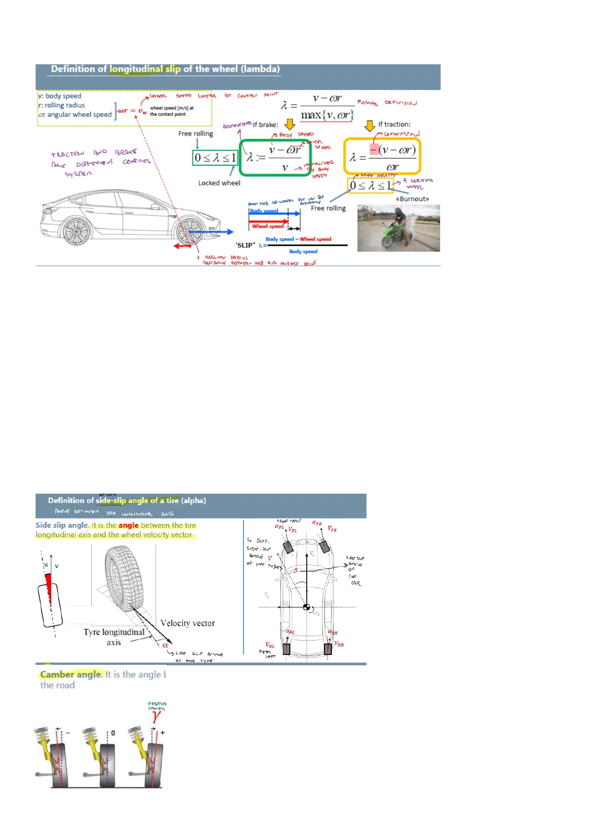
Definition of longitudinal slip of the wheel (lambda) Start with the definition of the v: body speed SOFFO LIMPAR AT CONTACT POINT v-cor r: rolling radius wr = Vw the contact point four : max{v, or} fundamental variable DEFINITION of this chapter, the 2= @: angular wheel speed wheel speed [m/s] at FORMAL If traction: ADIMENTIONAL If brake: Free rolling BODY SPEND longitudinal slip of the SPEED cor TRACTION AND BRANE v- or 0≤2≤1 2= -(v-(or) ARE DIFFERENT CONTROL wheel. We have the body speed (any point SYSTEM My BODY SACCO of the chassis has the Locked wheel A LUCKGO WHEEL same body longitudinal FROM HOB OF WINKEL POT CAN BE «Burnout»> AMYVANONE velocity, V), we have Body_speed Free rolling the rolling radius (R, Wheel speed the radius between the "SLIP" 2= Body speed - Wheel speed hub and the contact Body speed Y ROLLING RADIOS point, because of the DISTANCE BETWEEN HUB AND CANTERS POINT compression of the wheel of the tire it's slightly smaller than the non-rolling radius) and we have the angular speed (the rotational speed of the wheel). If you multiply omega times R, you get Vw, a linear wheel speed, it's a meter per second at the contact point.

Essentially we have two linear velocities, meter per second, the body translation velocity and the velocity of the wheel at the contact point, we call them V and Vw.

Longitudinal slip of the wheel is lambda, this quantity is body speed minus wheel speed normalized by body speed. The formal definition is this one lambda is V minus omega R divided by the maximum between V and omega R. This definition has two different instances, one is if break, one is if traction. If break the maximum is V: if the wheel is locked, the omega R is zero and you have some V. If traction, the max is omega R: the burnout is a classical extreme situation in traction, no movement, V is zero, omega R is bigger. Keep in mind that traction and breaking are usually two different design domains, so there is a traction control system, it's a control system, and there is a breaking control system. So, typically if you are a traction control designer, you don't want to keep all the negative quantities, so we put the minus and we go back to all positive quantities, but it's a conventional minus. Lambda is adimensional, because it's a normalized quantity, is speed over speed, so adimensional, and being normalized, lambda is restricted between zero, including zero and one, including one. Notice that zero is the so-called free rolling, that means that the body velocity is exactly the velocity at the peripheral point of the wheel, means that you are not breaking, you are not accelerating. And one is the extreme when you have a block wheel, a lock wheel. If you have a lock wheel, the car is moving anyway, even though the wheels are locked, so omega R is zero in a locked wheel, and then you have V over V, which is one.

Definition of Side-Slip Angle of a Tire

Definition of side-slip angle of a tire (alpha) ANOLE BETWEEN TIME COMEITUDINAL AXIS @FR Side slip angle. dt is the angle between the tire longitudinal axis and the wheel velocity vector aFL . VFL 4 DIFF. VER FRONT -UPET SIDE-SLIP AMORE V ¡a OF THE TYRES SIDE SUP JONGLE OF > CAR V The second very important variable, this --- ..... Tyre longitudinal Velocity vector CRL axis is super important in chapter three, is the definition of side slip angle of the VRI VRR tire. It is the angle between the tire LY SIDE SLIP AMUE REAR UPET OF THE TYRE longitudinal axis and the wheel velocity Camber angle. It is the angle } vector. For tires we have four side slip angles, keep in mind that the car itself has one side slip angle, which is called typically beta.

Camber Angle of the Tire

the road POSITION CAMER Y 0 + The third parameter, not so important, is the camber angle of the tire. It is the angle between the tire vertical action and the direction orthogonal to the road. It's called gamma. Ideally a car should always keep a zero-camber angle in any condition.

Tire-Road Contact Forces and Friction Coefficients

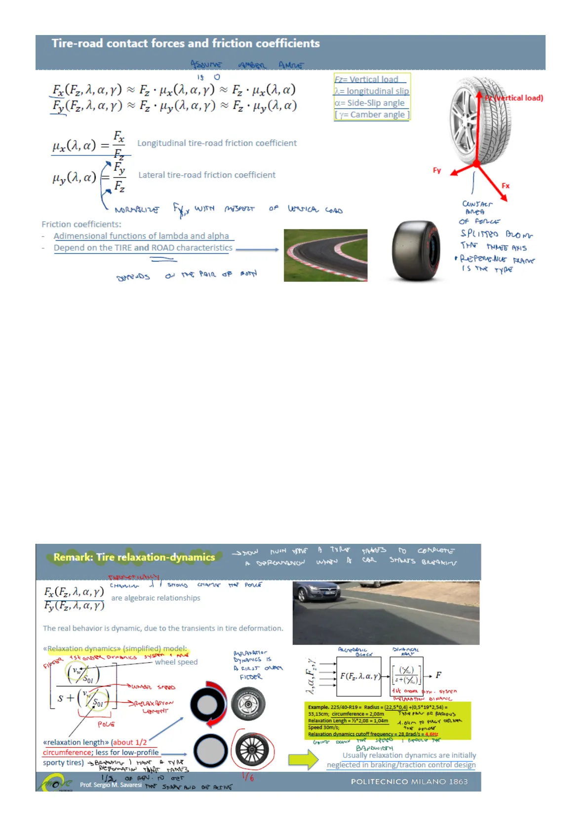
ASSUME AMBER AMUE 15 0 Ez= Vertical load Fx(F2, λ. α,γ) ~ F2 . μχ (λ, α,γ) ~ F2 · μχ (λ, α) Fy(F2, λ, α, γ) ~ F2 ' Hy (λ, α,γ) ~ F2 ' μy (λ, α) 2= longitudinal slip a= Side-Slip angle [ y= Camber angle ] Fz (vertical load) Hx(1,a) = Fx Longitudinal tire-road friction coefficient ₣ Fy Lateral tire-road friction coefficient Fz NORMALIZE FX WITH RESPECT OF LOSICAL CORD CONTACT AREA Friction coefficients: - Adimensional functions of lambda and alpha - Depend on the TIRE and ROAD characteristics DEPENDS ON THE PAIR OF BOTH OF FORCE SPLITTES ALONE THE THREE AXIS · REFERENCE FRANCE IS THE TYPE At the contact point, which it's a small area of contact, there is one vector force, which is exchanged between the road and the tire. This force usually is split along the three axis, and the reference frame is the tire. FY, FX, FZ are the three components in the tire reference frame, not the car reference frame, because the tire can steer for instance. You split the force into a longitudinal component, FX, which is useful to accelerate or break, the FY, the lateral, which is useful to turn and FZ, which is the load. FX and FY are functions of four variables, and the four variables are the vertical load, FZ, the longitudinal slip, the side-slip angle and the camber angle.

We can make a couple of approximations: The first approximation is FZ can be taken out and the relation is linear, so it's a sort of scaling factor. Fz that multiplies the remaining function, remaining function is called mu X or mu Y. Finally, we can make an additional approximation and negoct the camber angle, assuming is zero. We can say that FX is FZ that multiplies mu X function of lambda and alpha, same story for FY is FZ multiplying mu Y function of lambda and alpha. Finally, if you divide FX by FZ and FY by FZ, what you find is this function that we call mu X and mu Y and this function is called the longitudinal or the lateral tire road friction coefficient. So, mu X function of lambda and alpha, longitudinal slip and lateral slip is the longitudinal tire road friction coefficient, the same for the lateral friction coefficient.

The friction coefficient are adimensional functions because it's a normalization force over force. Notice that FZ is a normalizing factor, we normalize FX with respect to the vertical load, normalize FY with respect to the vertical load. It's the pair tire road that gives you a friction coefficient, you can have a tire with a very high friction coefficient on a type of road and a very low friction coefficient on a different road.

Tire Relaxation-Dynamics

Remark: Tire relaxation-dynamics MUCH THE A TYRE JAMES TO COMPLETE CHAMIMA 1 Strong CHIAMA MAS FORCE Fx (F2, λ, α, γ) are algebraic relationships Fy(Fz,À, a, Y) The real behavior is dynamic, due to the transients in tire deformation. «Relaxation dynamics» (simplified) model: ALGEBRAIC BLOCK DINAMICAL RALF FISKER - wheel speed RELAXAMON DYNAMICS IS A FIRST ORDER FILDER λ.α, F.,y. F(F2, λ. α, γ)} s+(5%) S + SOL SRELAX ASYON LEMENT Example. 225/40-R19 = Radius = (22,5*0,4) +(0,5*19*2,54) = 33,13cm; circumference = 2,08m TYME PAN OF RADIOUS Relaxation Lengh = 12º2,08 = 1,04m Speed 30m/s; Relaxation dynamics cutoff frequency = 28, Brad/s = 4.6Hz «relaxation length> (about 1/2 GOING DOWN THE SPEED I MOULE THE circumference; less for low-profile sporty tires) > BRAMMING I HAVE A TYRE DEFORMATION TANT TANES BANDWIDTH Usually relaxation dynamics are initially neglected in braking/traction control design IS OF REV. TO GET 1/6 POLITECNICO MILANO 1863 Prof. Sergio M. Savaresi THE SHAPE AND DE ALTIVE A DERENMANON WHEN A CAR STATS BREAKING 1st GRAPH DYNAMICS SYSTEM 1 mé SOL SWHEEL SPEED 1st ONDER DYN . SYSTEM RELAXATION DINAMIC POLE 1.04 M TO FULLY OUR NEW THE FORCE μη (λ, α) Fy FxWe are assuming that this relationship is algebraic, is instantaneous, if I change lambda, instantaneously, I get a new force. In practice, if these are the inputs and the output is the force, for instance, FX or FY, you have an algebraic block and a dynamical part. So, if you change lambda, for instance, if you change an input, you don't see instantaneously the effect on the output, but you see the effect with some dynamics. The dynamic behavior is approximated. It's a good approximation by a simple first-order dynamical system. It's called relaxation dynamics. The name tells you that it's due to the relaxation, so to the elastic behavior of the tire. The tire is an elastic object that has a relaxation dynamic. And the pole is VW over SOL, where VW is the wheel speed and SOL is the so-called relaxation length, about half of the circumference of the tire.

So, if you take a normal tire, roughly this relaxation length is half of the circumference, if you have a sport tire, the relaxation length is much smaller, it can be 1-6th of the tire. Only after the full deformation, you have the full force delivered by the tire. I start breaking, it takes half a revolution, the tire to modify the shape and give you the full force. If you have a stiff tire, a sport tire, in just 1-6th of the revolution, you get the full force. So, this is another point where sport tire is faster, you get immediately the force.

Let's take a tire, which is a-225-40-19. Notice that the radius is done by 2 parts, the rim and actually the tire. For the tire part you have to take 22.5 centimeters multiplied by 0.4. The rim part of the radius is simply 19 inches, which is the diameter, divided by 2. Inches, unfortunately. Unfortunately, our 19 are inches. Overall, the result is 33 centimeters, 33 centimeters is the radius of this type of tires, and the circumference is very easy, you get 2.08 meters. If the relaxation length is half of the circumference is 1.04 meters, so it takes 1.4 meters to fully deliver the force. So, let's assume that the speed is 30 meters per second, it's a bit more than, let's say, 100 kilometers per hour, means that the bandwidth of the relaxation length is 4 hertz.

Is it big numbers, small numbers? Well, consider that the bandwidth, we will see the bandwidth of an ABS, is a few hertz. So, in this case is interacting, you should take in consideration these dynamics. If you go down the speed, the bandwidth gets smaller and smaller, and so becomes more and more interacting with your control system. If you go high speed, the bandwidth of the relaxation dynamics become higher and higher, so you have a more decoupling between, let's say, the control system dynamics and this type of dynamics.

This is another very typical question of the exam: describe the phenomenon of relaxation dynamics and describe the main parameters of relaxation dynamics. You describe the phenomenon, you say this is the approximation, is first order filter and blah blah blah.

Contact Forces: Longitudinal Friction Coefficient

Fx= PZ- My Contact forces: longitudinal friction coefficient In this slide, you can 0" sideslip curve (1x (1, 0)) = all-longitudinal forces STRAIGHT ON HIGHWAY O SLIP IS WITH NEUTRAL - ONLY AERODINAMICAL PORLES see the shape of mu X, so the longitudinal friction coefficient and SHAPE Mx IN CUNCTA NO SLIP , MO CORLÉ 1.2 OR LONG. SHIP 15% NO VISIBLE then mu Y, as a TUE COPT MOMS SIDE - SLIP μα (λ, α) Example of dry-asphalt, with high-grip tire TURNING / STEENML 1.0 If there is no slip, the longitudinal force is zero 8º function of the 0.8 ANZ-LE 16° SJOK $ LIP Force increases linearly up to values of 2. of PEEK GOVE DOWN HIGHER about 0.1-0.15 longitudinal slip LONGISLAND SUIT lambda. Red line is mu 0.6 increasing Beyond the maximum: slope sign changes (!) tire side slip angle X lambda zero. We set 0.4 POINT YOU CAN'T USE LESS the side-slip at zero and Pron This Increasing side-slip angle: - Reduction of longitudinal force you go, you get the red 0.2 - The maximum point moves forward curve just to be clear, longitudinal friction co-efficient ux 0 this is the classical 0 0.1 0.2 0.3 0.4 0.5 0.6 0.7 0.8 0.9 1.0 «brush» model GOOD ASTHALS longitudinal slip situation when you are, when you go straight on the highway, so you are not turning. Dry asphalt with a good high grip tire is 1.2. If you are beyond one, it's a really high grip, if you go below one, there is something wrong, wet, snow, ... So, one means if you push one kilogram down, you get one kilogram maximum longitudinal friction. Red line, first of all, no slip, no force. If you have no slip you can't break and you don't have any traction force. The first part of the curve is very steep, so with just a small amount of slip you get a significant increase of the longitudinal friction coefficient. Remember that the force fx is simply fz times mux. At some point you have a peak, this peak is typically, in this case, is at 15%, notice that 15% slip is not visible by a visual inspection. Unfortunately, from this point on, the curve goes down, change sign and start going down. The brush model gives you the idea that, if you push the brush a bit, the hair of the brush actually follow you. At some point, if you push too much, they refuse to follow and then they are released.