Practical guide to digital elevation models of the seafloor

Ulster University School of Geography and Environmental Sciences

Ulster University SCHOOL OF GEOGRAPHY AND ENVIRONMENTAL SCIENCES ULSTER UNIVERSITY MODULE EGM518 PRACTICAL 7: DIGITAL ELEVATION MODELS (DEMS) OF THE SEAFLOOR

Aim of the Practical

To gain confidence in interpreting high-resolution bathymetric data derived from multi-beam echo-sounder surveys, to derived secondary products from the primary data and to start building your ArcGIS project for the underwater remote sensing assignment.

Practical Activities

In this practical you will:

1. Render digital elevation models (DEMs) from MBES bathymetry data
2. Derive secondary products from DEMs: (i) hillshade models, (ii) slope maps and (iii) profiles
3. Use focal statistics to generate rugosity indices and residual relief models
4. Explore point cloud data and render shipwrecks in 3D

EXERCISE 1: DOWNLOAD AND EXTRACT THE PRACTICAL DATA

The data for practical 1 are available for download from the EGM518 Blackboard site. The ZIP file contains numerous files, of which the important data files are:

• bl_bathymetry.img: multi-beam bathymetry data (raster data)
• bl_backscatt.img: multi-beam backscatter data (raster data)
• Ireland.shp: Irish Coastline (shape file, vector data)
• bl_sediment.shp (sediment samples, vector data)
• bl_wrecks.shp (shipwreck database, vector data)

Data Download and Storage Steps

1. Create a new folder on your external hard drive (HD) or OneDrive where you will store the data for the practical classes and assignment. I suggest you name this folder with a name that makes sense - e.g. EGM518_URS indicating the module code and module the component.
2. Download the file zip to the newly created folder on your external hard drive (HD).
3. Extract the contents of the zip file to the folder.

Over the next six weeks, you will use these data in the practical sessions and to complete the assignment. You therefore need to bring the HD with you to all sessions.

EXERCISE 2: GENERATING AND EXPLORING SEAFLOOR DEMs

A digital elevation model (DEM) is a 3D computer-generated representation of a surface created from a terrain's elevation data. In marine applications, the DEMs we use today are usually derived from multibeamechosounder data. A DEM can be represented as a raster (a grid of squares) or as a vector-based triangular irregular network (TIN). The TIN DEM dataset is usually referred to as a primary (measured) DEM, whereas the Raster DEM is referred to a secondary (computed) DEM. In exercises 1, 2 3 and 4, you will use a Raster DEM, and in exercise 5 you will use a vector (point cloud) DEM. The difference between the two should be very obvious by the end of this practical.

Adding and Interpreting Bathymetry Data

1. Add the bathymetry layer to your project by selecting the Add Data icon under the Map tab
2. For the remainder of this practical session, we will concentrate on the bathymetric data.
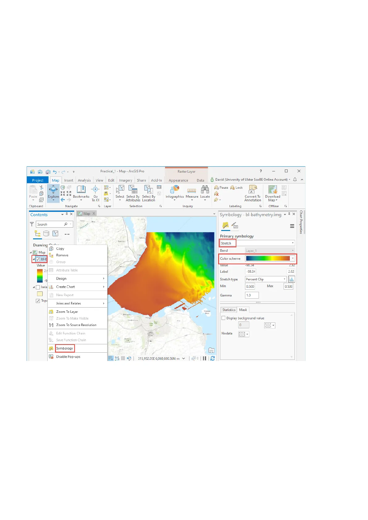
3. By default the raster layer representing the bathymetry appears in grey scale (256 shades of grey). To aid interpretation of these data, you will now change the colour scale of the bathymetric data. Right click the depth layer > Symbology. On the symbology pane select stretch as Primary Symbology. Click the drop down menu beside Colour Scheme to change the Colour Ramp to a rainbow colour-scale (cold colours representing deep values, warm colours representing shallow values). Can you see how using colour palettes to render the bathymetry can aid interpretation?

٠ ٥٠٠ Practical_1 - Map - ArcGIS Pro Raster Layer ? X Project Map Insert Analysis View Edit Imagery Share Add-In Appearance Data David (University of Ulster ScoBE Online Account) . ^ ni Pause & Lock A Paste Explore Bookmarks Go To XY Select Select By Select By Attributes Location Infographics Measure Locate Convert To Annotation Download Map - Clipboard Navigate Layer Selection F Inquiry Labeling Offline L Contents + 4 X Map X Symbology - bl-bathymetry.img - 4 x Y Search a = Chart Properties Map Remove V bl-b Group Value -98.34 2.92 2. Attribute Table Label -98.34 2.92 Design Stretch type Percent Clip Irela Create Chart Min 0.500 Max 0.500 Gamma 1.0 Top Joins and Relates Statistics Mask O Zoom To Layer Zoom To Make Visible Display background value 1:1 Zoom To Source Resolution 0 Edit Function Chain Nodata Save Function Chain Symbology Disable Pop-ups Giro Primary symbology 200 . Stretch Drawing O Copy Band Layer_1 4 Color scheme - Value New Report 315,952.05E 6,068,600.56N m v | 0 |||

Layer Naming and Geodatabase Management

4. Top-tip: After a few weeks of practicals, you will have created tens of layers. Naming convention is very important in Arc, so please give each layer a meaningful name as you go along, as each of the layers you create will be needed in the future in other practicals and when writing your report. The other thing to remember is to write your new rasters and vectors to the geodatabase you are saving your entire project in. This will maintain the links in your project.

Generating Hillshade Surfaces

5. We will now artificially illuminate the offshore landscape (i.e. create a virtual sun) to further aid interpretation. To illuminate the bathymetry, go to ArcToolbox (Under Analysis tab > Tools >Toolboxes). Select Spatial Analyst Tools > Surface > Hillshade. When the dialogue box opens, choose the depth layer as the input raster and leave the Azimuth and Altitude at the default values. An azimuth value of 315 with an altitude value of 45 means you are going to illuminate the offshore landscape with a sun placed at 315° (in the northwest) at an angle of 45° off the horizon. Give an output raster name e.g. HS and save within your geodatabase. Click 'Run' - it will take a few minutes to generate the hillshade surface. Once created the display can be enhanced by right clicking the layer > symbology and change the stretch type to 'Standard Deviation'5.00=

EGM518 URS Practical 1 - Map - ArcGIS Pro Raster Layer ? X Project Map Insert Analysis View Edi Imagery Share Add-In Appearance Data Not signed in To Cut ¡¡ Pause 28 Lock A Paste Explore Bookmarks Go Basemap Add Add Select Select By Select By Infographics Measure Locate Convert To Annotation Download Map + Copy Path To XY Data . Preset Attributes Location Clipboard Navigate Layer Selection Inquiry Labeling Offline L + 4 x Map X Symbology - HS + 4 X Y Search a B90 = Primary symbology Drawing Order Band Band_1 Map 145 m Color scheme Value Value 0 254 Label 0 254 0 Stretch type Standard Deviation Number of standard deviations 2 bl-bathymetry.img Value Gamma 1.0 2.92 Statistics Mask Ireland Lighthouse Island Statistics Dataset Options World Topographic Map Min O Max 254 46 m 1:136,305 |38,063.68E 6,069,133.85Nm . | 0 |||

Combining Renderings for Enhanced Interpretation

6. Now, we want to combine both of these renderings of the offshore landscape into one final rendering of the offshore landscape. To do this, we put the hillshade surface behind the colour-coded bathymetry and make the colour-coded bathymetry semi-transparent to allow the illumination to show through. First of all, drag the illumination layer below the colour bathymetry layer in the Contents. Now click the colour-coded bathymetry layer in the contents to make it active, go to the 'Appearance' tab and change Transparency to 40%. You can type 40% in the box or alternatively use the slide rule.

5.000 EGM518 URS Practical 1 - Map - ArcGIS Pro Raster Layer ? X Project Map Insert Analysis View Edit Imagery Share Add-In Appearance Data Not signed in " < In Beyond <None> Out Beyond <None> 4 Symbology Stretch Type + Resampling Type - Band Combination Enhancement Rotate Visibility Range Effects Rendering Contents +4 X Map X B90 Search B149 Drawing Order Map bl-bathymetry.img Value B90 A2 2.92 -98.34 SH Value 254 0 Lighthouse Island Ireland Groomsport Copeland Island World Hillshade 46 m A2 A 1:136,305 322,447.98E 6,076,454.84N m v Y Selected Features: 0 | || |

Finalizing the Digital Elevation Model

7. You should now have an artificially-illuminated digital elevation model (DEM) representing offshore bathymetry for your assignment.

World Hillshade Groomsport Copeland Island A Contents A2 141 m Stretch 4 HS 254 A2 40.0 % ¢ DRA Masking " 500.0 ms 1 145 m A2 World Topographic Map Warren Re -98.34 + i Copy8. Now play about with creating hillshades from different orientations to see how this can help and hinder your interpretation of the landscape. Try one at an azimuth of 45° (in the northeast) at an angle of 45° and look at the differences in the way the benthic terrain is rendered. This is most obvious around the bedforms. This is an important thing to consider when interpreting data ... hillshading can often bias our interpretations of geomorphic data - termed 'azimuth bias'.

EXERCISE 3: DERIVING SLOPE MAPS

Creating a Slope Map

1. Create a slope map from the depth layer using the Slope tool (this is in ArcToolbox under Spatial Analyst Tools > Surface). Use the DEGREE option for the Output measurement. After naming output raster, click 'Run'.

Changing Slope Data Color Scale

2. By default the raster layer representing the slope appears in brown scale. To aid interpretation of these data, you will now change the colour scale of the slope data. Right click the slope map > Symbology. On the Symbology pane, under Primary Symbology select Stretch. Under Color Scheme change the Colour Ramp to a rainbow colour- scale (cold colours representing shallow gradients, warm colours representing steep gradients).

5.000 EGM518 URS Practical 1 - Map - ArcGIS Pro Raster Layer ? X Project Map Insert Analysis View Edit Imagery Share Add-In Appearance Data Not signed in. ^ History Python ModelBuilder Environments Tools Ready To Feature Use Tools - Raster Analysis - Analysis Analysis Gallery - Analysis - Network Geostatistical Business Wizard Analysis tx fx Function Raster Functions - Editor Workbench Geoprocessing Portal Tools Raster Data Intero ... Contents +4 X Map X Symbology - Slope +4 X T Search a = Primary symbology Drawing Order Map AZ Color scheme Value Value 0 61.6969 61.6969 Label 0 61.6969 0 Stretch type Percent Clip Min 0.500 Max 0,500 D bl-bathymetry.img HS Groomsport Gamma 1.0 Ireland World Topographic Map Statistics Mask World Hillshade 1:212,976

Interpreting Slope Maps

3. Can you see how using colour palettes to render the slope map aids interpretation? Spend a few minutes examining where the steep and shallow gradients are located. How do these areas relate to the trends in bathymetry?

EXERCISE 4: EXPLORING WRECKS IN 2D: 'NORMAL' RESOLUTION DATA

Conventional multibeam echosounder surveys for hydrographic purpose result in rasters output at 2 m resolution (i.e. each pixel measures 2 x 2 m). In this exercise, you are going to investigate the known locations of shipwrecks in the study area (recorded by the UK Hydrographic Office) against their signatures in the multibeam echosounder bathymetry data.

Loading and Visualizing Shipwreck Data

1. Turn on the bathymetry and hillshade layers and turn off all other layers in your ArcGIS project. 2. Load the shipwrecks shapefile using the 'Add Data' icon under the Map tab. You might want to change the symbol type and colour (double click symbol in Contents) so the wreck sites are easy to identify.