Industrial Organization: Market Power, Efficiency, and Asymmetric Information

Market Power

The Market Power is the ability to set prices above cost, mainly marginal costs (const of producing one extra unit). For a Firm that means greater profits and greater value. From a Social Welfare pov the implication is inefficient allocation of resources, increase in costs and firm that spend resources trying to influence policy makers.

Efficiency and Welfare

Can we reallocate resources to make some individuals better off without making others worse off?

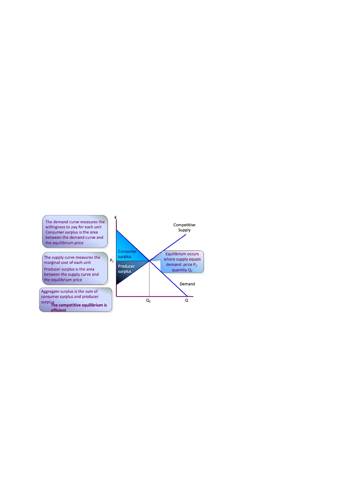
€ The demand curve measures the willingness to pay for each unit Consumer surplus is the area between the demand curve and the equilibrium price Competitive Supply Consumer surplus The supply curve measures the marginal cost of each unit Pc Producer surplus Equilibrium occurs where supply equals demand: price Pc quantity Qc Producer surplus is the area between the supply curve and the equilibrium price Demand Aggregate surplus is the sum of consumer surplus and producer surplus The competitive equilibrium is efficient Qc Q consumer surplus: difference between the maximum amount a consumer is willing to pay for a unit of a good and the amount actually paid for that unit producer surplus: difference between the amount a producer receives from the sale of a unit and the unit cost total surplus: consumer surplus + producer surplus

Entry and Exit

A restriction in a market entry will increase the price above the competitive level, that cause a dead weight loss in the market.

Barriers to Entry

Kind of Barriers to Entry: set up costs, patents, exit costs + economies of scale - product differentiation - access to distribution channels - government policies

Monopoly

A firm is a monopoly if it is the only supplier of a product in a market where there are no close substitutes.

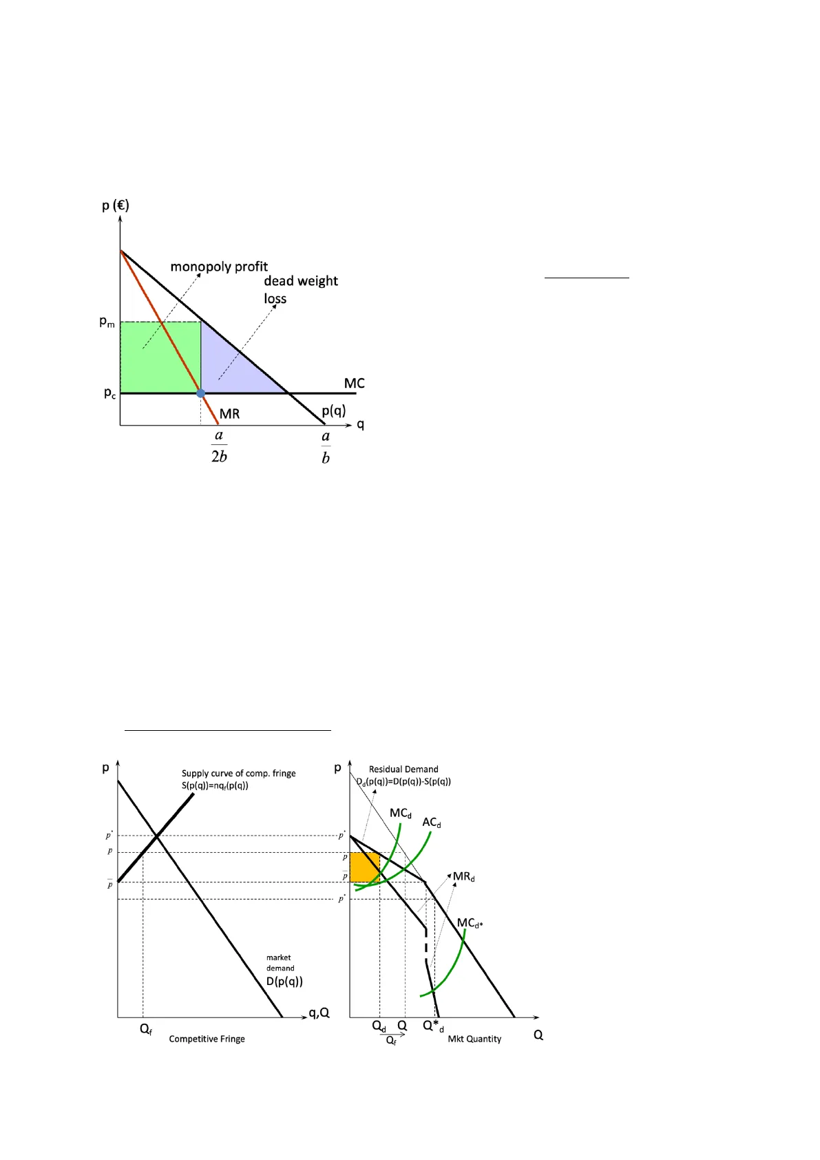
p (€) monopoly profit dead weight loss Pm MC Pc MR p(q) · q a a 2b b A monopolist can set the price without being afraid of being undercut by its rivals. Since the firm is a price setter, it faces a downward-sloping market demand. It can raise its price above marginal cost. MR>0 if the demand curve is elastic. MR<0 the demand curve is inelastic. A monopolist never operates on inelastic portion of the demand curve because it isn't possible to meet a profit maximizing condition.

Dominant Firm with a Competitive Fringe

There are markets with a Dominant Firm (price setter) vs several small competitive firms (price takers).

Dominant Firm Characteristics

A firm may be dominant: - To have lower costs (more efficient) than fringe firms - To have a superior product Whether or not a dominant firm can exercise full market power in the long run it depends on the number of firms that can enter the market and how are their relative production costs.

p Supply curve of comp. fringe S(p(q))=nq}(p(q)) p Residual Demand Da(p(q))=D(p(q))-S(p(q)) MCd AC d -p p 2 «MRd 4 p MCd* market demand D(p(q)) q,Q 1 Q Competitive Fringe Qf Mkt Quantity Q When P* and P the residual demand = 0 Qd is the quantity produced by the dominant firm, Qf is the quantity produce by the small firms to fill the space with the demand. p p p

Monopsony and Factor Market

In a monopsony there is only one buyer of a good in a given market that wants to buy at the lower possible price.

• vertically integrated: a firm that participates in more than one successive stage of the production or distribution of goods or services.

Marginal Revenue Product of Labor (MRPL)

MRPL: Marginal Revenue Product of Labor is the extra revenue from hiring one more worker: MRPL = MR . MPL In a COMPETITIVE MARKET a firm faces an infinitely elastic demand for its output at the market price so MR=p and: MRPL = p . MPL The firm maximizes its profit by hiring workers until the marginal revenue product of the last worker exactly equals the marginal cost of employing that worker. That's until when: MRPL= p . MPL = W The wage line is the supply of labor the firm faces. The MRPL is the firm's demand curve for labor.

Monopsonist's Profit Maximization

MONOPSONIST'S PROFIT MAXIMIZATION: A monopsony chooses a price-quantity combination from the industry supply curve that maximizes its profit. Suppose a monopsonist selling at price P in a competitive market: n = P.Q(X) - P (X).X Profit = tot revenue - tot expenditure Maximizing for X we obtain the following condition: MRP .= P(OQ/>X) = ME = P (X) + P.'.X x Px (X) rearranging: (MRP -P_) /Px = 1/s3, where & is the supply price elasticity(MRP -P ) /P = 1/8 x x' is a measure of market power (Lerner index) The larger & is, the lesser the price reduction that the buyer is able to impose. If the supply is very elastic (horizontal), a price reduction causes a more than proportional quantity reduction.

Is Monopsony Always Detrimental?

IS MONOPSONY ALWAYS DETRIMENTAL? The downward pressure the dominant buyer exerts upon producers forces the less efficient among them to merge, achieve economies of scale, cut costs, or exit the market, leaving the more efficient ones behind.

Bilateral Monopoly

BILATERAL MONOPOLY: Price, Costs (£) Monopoly outcome: Xs Monopsony outcome: XB Cooperative outcome: x* maximizes joint profits; price between H and L MFC H MC=Sc Ws AC WB L AVP=Dc MMRP MRP 0 XS XB X Xc Factor (Quantity) MRP = marginal revenue product MMRP = marginal of the marginal revenue product MFC = marginal factor cost (or ME marginal expenditure) Xs the seller is dominant, he set the price -> maxTt : MMRP = MC Xb the buyer is dominant -> maxTt : MRP = MFC max overall TT : MRP = MC

Price Discrimination

Strategy that allows to increase profits taking away as much surplus as possible from consumers.

Conditions for Price Discrimination

To be able to practice price discrimination the monopolist must: - Learn information about consumers - Separate the different demands and markets (also geographically) - Different prices are charged to different customers based on their willingness to pay

Perfect Price Discrimination (First Degree)

PERFECT PRICE DISCRIMINATION (FIRST DEGREE): Perfect price discrimination: the monopolist charges each customer their reservation price Profit: gap between reservation price and ATC PM Monopolist will produce at the efficient level ATC MC = ATC Demand (MR for the discriminant monopolist) QM QPD MR 4 · Firms try to sell each quantity at the maximum price the consumer is willing to pay (reservation price). . The monopolist is able to steal all the consumer's surplus · Maximum Tt condition: MR=MC · Marginal consumer: reservation price (WTP) = MC = P . Optimal allocation of resources Is perfect discrimination possible? The information requirement appears to be insurmountable, even if not in all the cases. No arbitrage is less restrictive but potentially a problem.

Quantity Discrimination (Second Degree)

QUANTITY DISCRIMINATION (SECOND DEGREE): € Second-degree price discrimination is pricing according to quantity consumed -- or in blocks. P - I P2 MC P 1 D MR Q1 Q0 Q2 Q3 Quantity 1st Block 2nd Block 3rd Block It's a nonlinear pricing scheme Block-pricing schedules: charge one price for the first unit (a block) of usage and a different price for subsequent blocks. Each subsequent block is sold at a lower price (WTP decreases) down to P=MC

Third Degree Price Discrimination

THIRD DEGREE PRICE DISCRIMINATION: This form of price discrimination divides consumers (with different demand curves) into two or more groups with different price elasticities. It is the most prevalent form of price discrimination. Max TT = P (q ) q + P (q2)q2 - C(q +q) FOC: MR = MC MR2 = MC MR = MR2= R2 = MC Relative price: D P /P2 = (1 + 1/E 2) / (1 + 1/E ) D higher price will be charged to the group with lower demand elasticity P P P P1 P2 D1+D2 MR1 D1 MR2 D2 MRT q1 q2 q1+q2

Non-Linear Price Scheme

NON-LINEAR PRICE SCHEME: Two-part pricing is an example: charge a quantity-independent fee plus a per unit usage charge. (ex. Membership to athletic clubs). The idea is to increase the monopolist profit at the expenses of the consumer surplus. . Total surplus is maximized P a .No other production level allows a higher profit to the monopolist PM B ·Maximum allocative efficiency is achieved (same asperfect competition) C+& MA C C ·If P>c, demand Q is lower (and therefore also n) (area ) D MR QM Q Qd Q MCn = (b1 + Cq1 + b2 + Cq2)-C(q1 + q2) P P1 c MR1 D1 MR2 D2 q1 q1 92" q2 The pricing scheme differs in the fixed part: b2>b1 o The monopolist can introduce only one pricing scheme (one fixed part for both types) 1. Apply b1: both consumers enter the market (why?) 2. Apply b2: only type 2 enter the market (why?) 3. Apply b>b2: nobody buys anything 4. b1

Product Differentiation

Most firms sell more than one product. Preference for a specific brand is determined by: - Availability at a closer store - Superior post sales services - Alternative brands are unknown - Perceived superior quality

Horizontal Product Differentiation

HORIZONTAL PRODUCT DIFFERENTIATION: The Spatial Model (Hotelling) is useful to consider pricing, design and variety. The differentiation is considered: - "Location" can be thought of in: o Space o Time o Product characteristic - Consumers prefers products that are "close" to their preferred types in space, time and/or characteristics E.g. assume N consumers living equally spaced along 1km long street, the monopolist must decide how best supply these consumers and where place his only one shop. Price Price P1 + tx P1 + tx V t t All consumers within distance x1 to the left and right of the shop will buy the product Z= 0 X1 1/2 X1 Z= 1 Shop 1 N = nº of consumers n = nº of shops x = distance = 1 t = transport costs V = utility Consumers buy exactly one unit provided that price plus transport cost is less than V -> V >= P + txt represents the slope of the two curves: - If t is small the customer preferences aren't strong, the curve is flatter and so the seller can set higher prices - If t is high the consumer has a strong preference and so the prices will be smaller What if there are two shops? Price Price V V V - t/4 V - t/4 C C Z= 0 1/4 1/2 3/4 Shop 2 Z=1 Shop 1 The monopolist will coordinate prices at the two shops. With identical costs and symmetric locations, the prices will be higher than in the one-shop situation and they will be equal: P1 = P2 = P The shaded area represents the profit for each shop. Social Optimum: are there too many shops or too few? What number of shops maximizes total surplus? Total surplus = consumer surplus + profit Consumer surplus is total willingness to pay - tot revenue: NV - PN - T(N,n) Profit is tot revenue - tot costs: TT = PN - mN - nF Total willingness = NV - T(N,n) -mN -nF Price Price V V Total cost is total transport cost plus set-up costs Transport cost for each shop is the area of these two triangles multiplied by consumer density t/2n t/2n Z=1 z = 0 1/2n 1/2n Shop i This area is t/4n2 Total cost with n shops is, therefore: C(N,n) = n(t/4n2)N + nF = tN/4n + nF Total cost with n + 1 shops is: C(N,n+1) = tN/4(n+1)+ (n+1)F Adding another shop is socially efficient if C(N,n + 1) < C(N,n) This requires that tN/4n - tN/4(n+1) > F which implies that n(n +1) < tN/4F